Smooth optimisation of demand patterns in water distribution system hydraulic model

First published in Water e-Journal Vol 8 No 1 2022.

How an automated calibration method can achieve smooth demand patters in Water Distribution System hydraulic models.

DOWNLOAD THE PAPER

Abstract

This study proposes a new approach to obtain smooth demand patterns while calibrating water distribution system (WDS) hydraulic models using an automatic calibration method. The water usage patterns in a WDS vary throughout the day and night which is represented by demand multipliers. Through the calibration process, many parameters including demand multipliers are adjusted to minimise the difference between simulated and the observed data at the point of interest. This is achieved by minimising the objective function value. The demand multipliers in a 24-hour cycle sometimes become unsmooth and often a major difference between two adjacent demand multipliers is observed due to under or over calibration which is unrealistic. To obtain a smooth demand pattern, programming functions were incorporated with the calibration process. Two different approaches were investigated where in the first approach, the demand multipliers as sampled by the optimisation algorithm within their specified range were smoothed by a smoothing function and used the smoothed pattern in assessing the objective function value. In the second approach, the demand pattern was represented by a Fourier polynomials function and optimise the function parameters. The proposed method tries to keep a balance between minimum objective function and the smoothness of demand patterns. This approach was applied in calibrating the hydraulic model of a large WDS in South Australia and found to have the potential to ensure minimum objective function as well as smoothness of demand patterns. This method is suitable when there is insufficient field data available to create demand patterns rather estimating them through model calibration.

Introduction

Hydraulic models are frequently used in many areas including but not limited to analyse hydraulic states of a network system and to study development scenarios for planning and management, and hence act as a decision support tool to improve the system’s performance (Kara et al., 2016). A water distribution system (WDS) serving a variety of customers and the water usage or demand patterns associated with different types of customers are highly variable in space and time. The demand patterns in a WDS are classified as: (i) residential (ii) commercial and (iii) industrial (Letting et al., 2017). In a hydraulic model, the demand patterns are represented by introducing demand multipliers that relate to the change of water usage in a 24-hour cycle with respect to a baseline value. Hence, the hydraulic model is required to calibrate to ensure that it closely reproduce the observed patterns in the real system (Shen and McBean, 2010, Moradi et al., 2018).

The calibration of a hydraulic model is done by conducting multiple model runs to optimise several parameters including demand multipliers, pipe roughness, settings of various hydraulic components, etc. The number of parameters to optimise are quite large resulting in an increased search space, making it a considerably complex task. Among these parameters of a hydraulic model, some are highly uncertain in space and time. Kang and Lansey (2011) stated that pipe roughness and demand multipliers are the most uncertain parameters associated with a WDS hydraulic model because they are not practically measurable in the field. Hence, these parameters are fixed through the model calibration process. Over the years, many algorithms have been developed to minimise some of these issues in the optimisation process. Some offer the option to incorporate external functions into the hydraulic model to automate the calibration process.

WDS hydraulic model calibration can be considered as a non-linear and ill-posed optimisation problem (Do et al., 2016, Zanfei et al., 2020). Because several components of a WDS hydraulic model are controlled using simple and logical rules leading to break up the linear sensitivity of many parameters. Some parameters also show a composite sensitivity meaning changing their values may affect the sensitivity of other parameters. During the calibration process, parameter values are searched within the defined space and can take any values to satisfy the criteria of minimum objective function. Often the optimisation is heading to the path led by the sensitive parameters. This can lead to a considerable difference between two adjacent demand multipliers or irregular peaks if the search space is not carefully defined. Since the demand patterns in a WDS are highly uncertain, it isn't easy to define a narrow search space. Representing a more exhaustive search space can result in increased chances of irregular patterns and peaks.

The demand multipliers in a real WDS does not sharply rise or fall between two adjacent timestamps rather they change in a regular fashion. Hence using different methods, including pre-smoothing them before populating the model input file or expressing them as a function of time and optimising the function parameters, allows representing the pattern between two adjacent timestamps more practically. Therefore, the objectives of the study are: (i) to assess and incorporate the smoothness option into the calibration process and (ii) to calibrate the hydraulic model while maintaining the maximum smoothness of the demand patterns. This is a novel approach that allows to model and obtain realistic demand patterns hence, contributes to improve the hydraulic modelling application.

Materials and Methods

Study area

The case study selected was Tailem Bend-Keith (TBK) drinking water distribution system, which is in regional South Australia, approximately 80 km South East of Adelaide. It extends from Tailem Bend to Keith township with the major branches including Karoonda, Lower Lakes, Meningie, etc. The TBK system withdraws water from River Murray and treated at the Tailem Bend water treatment plant (WTP) using conventional treatment process (Hossain et al., 2020, Moradi et al., 2018, Hossain et al., 2021). The treated water is then pumped into the distribution network consisting of about 143 km long pipeline and several hundred kilometers of branch mains. Supervisory Control And Data Acquisition (SCADA) is used to monitor hydraulic and water quality data at several strategic locations in the distribution system. The schematic of the TBK distribution system is presented in Figure 1.

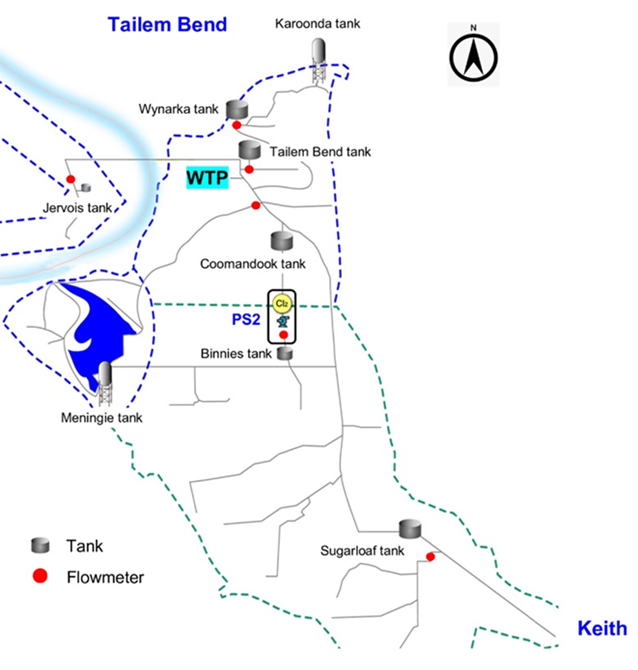
Figure 1. Schematic of the TBK distribution system in South Australia.

Modelling demand patterns

The demand patterns were modeled using a non-linear function/ multi-parameter curve. The position, spread and peaks of the curve to be adjusted through the calibration process. This will ensure a smooth pattern as optimising the demand multipliers directly often cause unsmooth or unlinked pattern between the subsequent demand multipliers or irregular peaks. Several functions were assessed and the Fourier n^th order polynomial was found to satisfactorily represent the demand patterns in a WDS. An n^th order Fourier polynomial has 2n+1 parameters which were included in the calibration process.

The Fourier polynomials represent a curve in terms of a linear combination of some basis functions. They can be expressed by either trigonometric function or exponential function. In the trigonometric form, the function is expressed as a combination of sine and cosine series. This way the original curve is decomposed by assigning a coefficient to each sine and cosine term that best represent the strong underlying repetition pattern and at the same time it corrects many other weaker repetitions by partially cancelling each other. The trigonometric expression of the Fourier polynomials is given in Equation 1.

Where a₀ represent a constant (intercept) term associated with the cosine term at i = 0, n is the total number of harmonics present in the curve and w is the frequency. The coefficients a_i, b_i are weights or scaling factors for each sine and cosine term in the equation. They indicate the strength of the underlying repetition patterns and the associated cycle-relative shifts from each other.

Hydraulic and calibration setup

EPANET, a public domain hydraulic modelling tool developed by the US Environmental Protection Agency (USEPA) was used to develop the hydraulic model (Rossman et al., 2020). It simulates the hydraulic behaviour in nodes and links by solving the mass conservation equation for each node and the energy equation for each link in the network (Muranho et al., 2015, Rossman et al., 2020). The data required to setup the hydraulic model and the calibration process includes GIS and SCADA data which were obtained from the South Australian Water Corporation (SA Water). Missing data were estimated using linear interpolation and the extreme values in the data were replaced with the closest sensible values. The total inflows and outflows during the study period were balanced by adjusting the base demands at all nodes using the SCADA flowmeter data at the available locations. This required re-adjusting the sampled demand multipliers by the optimisation algorithm such that their average value always becomes one. R programming language (RCoreTeam, 2019) was used to pre-process the data before passing to the model input file and PEST (Parameter Estimation), a non-linear optimisation tool was used to calibrate the model (Doherty, 2005). This is a model independent parameter optimisation tool, widely used in many surface and groundwater applications (Doherty and Skahill, 2006, Hossain et al., 2019, Hossain et al., 2021).

The Covariance Matrix Adaptation Evolution Strategy (CMAES), which is a global search algorithm was employed in parameter optimisation. The CMAES algorithm was first proposed by Nikolaus Hansen which has been proven to be suitable in optimising non-linear problem or searching the global minima in a rugged landscape (e.g. noisy, multi-modality, many local optima, etc.) (Hansen and Kern, 2004, Hansen and Ostermeier, 2001). CMAES involves an iterative procedure to minimise the objective function. At each iteration, possible candidate solutions are generated according to a multivariate normal distribution and ranked them by order. For the next iteration, the parameters of the multivariate normal distribution are updated based on the rank and the search space is adaptively increased or decreased.

As shown in Figure 2, different approaches were tried to obtain a smooth demand pattern. In the first approach (Figure 2a), the optimisation algorithm sampled the demand multipliers within the defined range. Prior to populating the model input file, the sampled demand multipliers comprising the demand patterns were smoothened by implementing the R programming codes and the model input file was populated using the smooth demand patterns. In the second approach (Figure 2b), the demand multipliers were represented by an equation and the equation parameters were optimised. Prior to each model run, the optimisation algorithm sampled the equation parameter values which were then passed to the programming codes to regenerate the smooth demand multipliers which then used to populate the model input file. Both procedures continue until the convergence criteria were met.

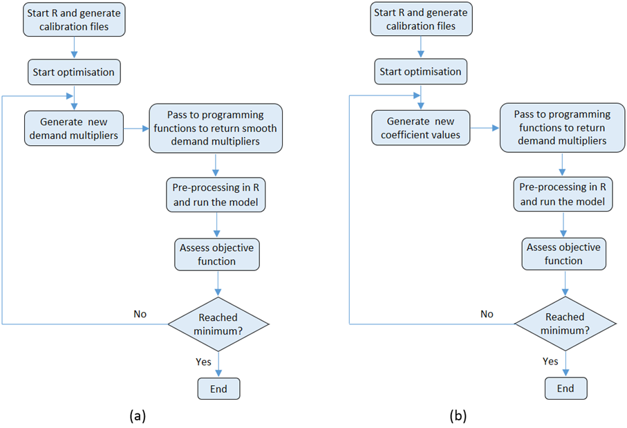
Figure 2. Flowchart of the calibration setup (a) smoothing the sampled demand multipliers prior to model run using a smoothing function by employing R programming codes and (b) representing the demand pattern using an equation and optimising the equation parameters.

The objective function used was to minimise the sum of square residuals between the observed and the simulated data which includes tank head and flow data at the points of interest. The convergence criteria to terminate the optimisation process were: (i) insignificant reduction of parameter values or objective function over successive iterations; (ii) convergence of parameters to their optimal values and (iii) exceedance of the maximum number of iterations (Doherty, 2005). Throughout the calibration process, the objective function was assessed, and the process terminates once there is no significant improvement of objective function between n successive iterations or any other convergence criteria is met. The calibration process requires running the model hundreds to thousands of times, consuming a considerable amount of time to complete the process. This was handled by employing parallel processing in a high-performance computing (HPC) environment.

Results and Discussion

The curve fitting approach found that a Fourier 6^th order polynomial can satisfactorily represent the residential demand multipliers while a 5^th order is adequate to represent the commercial demand. The R² value obtained in both fits were over 0.99 indicating a satisfactory fit. The 6^th and the 5^th order Fourier polynomials have thirteen and eleven parameters respectively to include in the calibration process. Though increasing the polynomial order improves the fitting, to be parsimonious, further increase of the polynomial order was not considered and the maximum fit with the minimum number of parameters was sought. Representing a curve with less parameters also reduce the solution space during optimisation by reducing the population size. Consequently, the number of model runs and the convergence time also decreased. Similarly, an increased number of parameters increase the convergence time by increasing the solution space. On the other hand, any further modification or transformation of parameters between the processes by the optimisation algorithm and the model run in an iteration loop may increase the non-linearity of the objective function with respect to the parameters representing the model and the convergence time increase.

The hydraulic model of the TBK system was developed and the parameters to be calibrated were defined. Figure 3 shows the initial values of the demand multipliers used in the calibration process, their upper and lower limits and the optimised demand multipliers obtained through the calibration process. The initial values and the upper and lower limits of the demand multipliers were obtained by analysing the SCADA data during the study period of February to March, 2021. The upper and lower limits of the demand multipliers were comparatively narrow between 10 pm to 6 am as the variation of water usage during this period was minimum. The global optimisation algorithm does not require any starting point rather the model is run using multiple start points and the objective function is assessed. However, providing an initial starting point can significantly decrease the number of model runs. It is evident from Figure 3a that calibration using the hourly/sub-hourly residential demand multipliers cause irregular patterns and many peaks. This is because optimisation minimises the difference between observed and simulated data and in doing so, the demand pattern may characterise poorly. On the other hand, while applying the smoothing function many irregular peaks disappeared and the resulting demand pattern is more similar to that observed in a typical WDS. The optimised commercial demand pattern is presented in Figure 3b which also indicates a smooth pattern when using the smooth function.

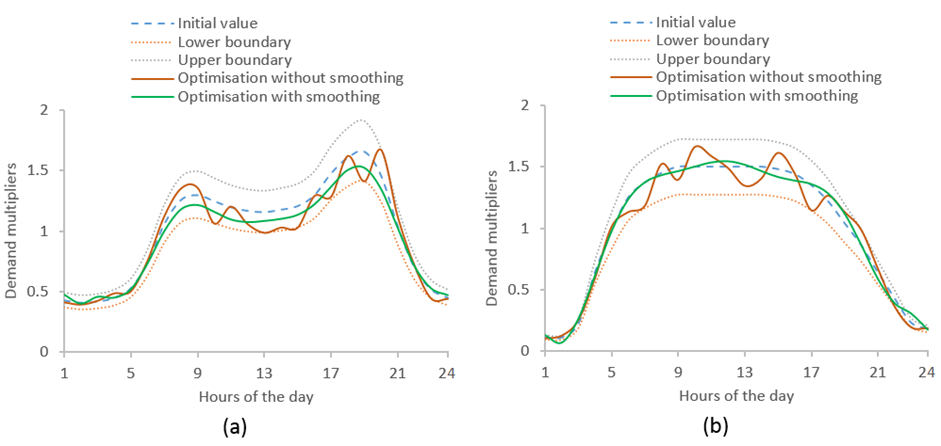Figure 3. Initial values of demand multipliers, their upper and lower boundaries and the optimised demand multipliers for (a) residential demand pattern and (b) commercial demand pattern.

The plots of the observed vs simulated tank heads for two different points located at Binnies and Meningie and a flowmeter located at pump station 2 (PS2) in the TBK distribution system are shown in Figure 4. The trend lines indicate that for both cases, (i) unsmooth demand patterns and (ii) smooth demand patterns, the model reproduces the observed data with a good level of accuracy. In the first case, the correlation between the observed and the model simulated heads at Binnies and Meningie tanks and flow at PS2 were 0.95, 0.88 and 0.80, respectively. The mean of the observed and the simulated tank heads at Binnies were 136.77 m and 136.76 m, and at Meningie were 42.53 m and 42.54 m, while the same for the observed and the simulated flows at PS2 were 57.19 L S^-1 and 55.92 L S^-1, respectively. For the second case, the correlation between the observed and the simulated tank heads and pump flow were 0.96, 0.89 and 0.79, respectively.

In contrast, for smooth patterns, the mean of the simulated tank heads at Binnies and Meningie were 136.82 m and 42.54 m while the same for simulated flow was 54.75 L S^-1 respectively. The standard deviation of observed flow at PS2 and simulated flow using unsmooth and smooth patterns were 55.8 L S^-1, 54.2 L S^-1 and 52.1 L S^-1 respectively. The minimum of observed and simulated flows was 0 L S^-1, while the maximum of observed and simulated flows for both cases were 190.5 L S^-1, 168.08 L S^-1 and 168.36 L S^-1 respectively. The percentage error of mean flow at PS2 for unsmooth and smooth patterns were 2.2% and 4.2% respectively. These statistics indicate that by incorporating the smoothing function in the calibration process, model can effectively describe the observed data.

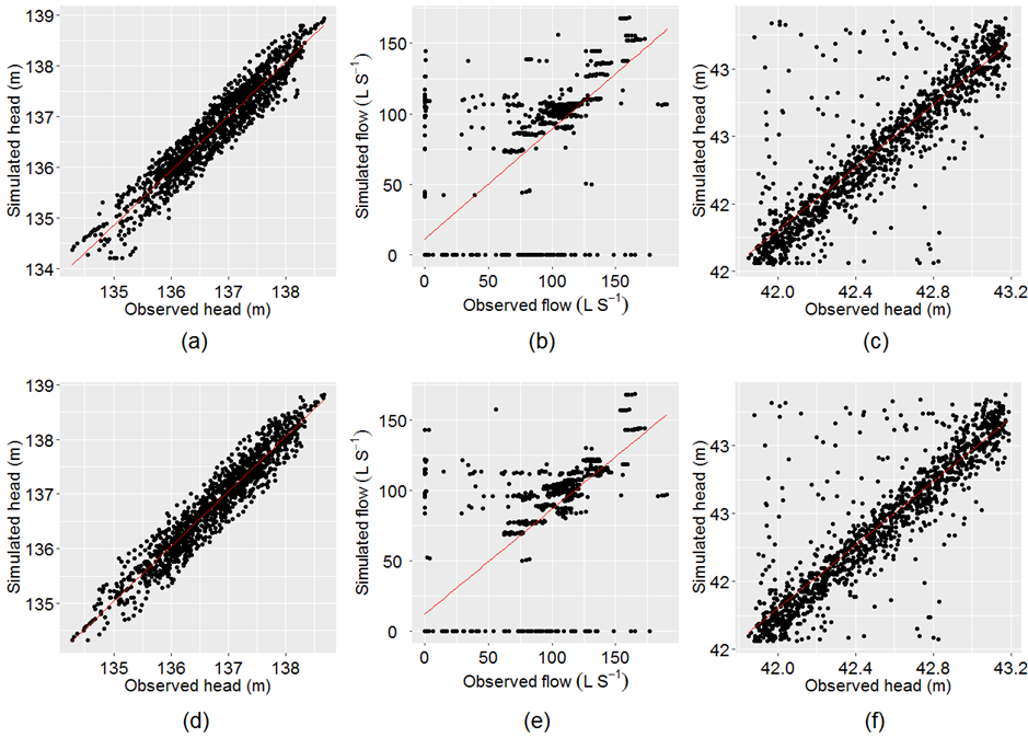Figure 4. Plot of the observed vs the simulated data using unsmooth and smooth demand patterns resulting from calibration (a) head at Binnies tank using unsmooth demand patterns; (b) flow at PS2 using unsmooth demand patterns; (c) head at Meningie tank using unsmooth demand patterns; (d) head at Binnies tank using smooth demand patterns; (e) flow at PS2 using smooth demand patterns and (f) head at Meningie tank using smooth demand patterns.

When calibrating a hydraulic model, often the smoothed demand patterns are created from the actual calibration patterns after the calibration has been completed. The smoothing is done using a smoothing function, and the resulting smoothed patterns can further increase the calibration objective function value. Therefore, smoothing them prior to passing to the model and assessing the objective function value during calibration can ensure smoothness and minimum objective function. Usually, in developing hydraulic models, field data are used to create demand patterns and scaling factors. In most cases water balance calculations are discrete (complete) and accurate enough to use real data. The exception is when there are gaps in the water balance calculation (i.e. a missing flow meter), or the calculated profile is highly irregular. The proposed method has the benefit to establish a smooth profile while maintaining the least error function. It may help to estimate the demand when a zone contains a missing flow meter or improve model usability by having a smooth profile. Current models sometimes have trouble converging a calculation when there is a significant step change in hydraulics; a smooth profile helps avoid this problem.

The calibration of a WDS hydraulic model is a considerably complicated task due to a large number of parameters involved in the modelling and calibration process, some of which are highly uncertain in space and time. Therefore, it is difficult to obtain a unique set of parameter values that correspond to the global minima, rather many different set of optimised values may lead to similar objective function. The best parameter set should be identified using the WDS modelling experience, and hence can be subjective. The method presented here can ensure minimum objective function by maintaining smooth demand patterns resulting from calibration. This approach used single residential and commerical patterns for each zone which represent average pattern from the relevant users in that zone. If individual customer water usage data are available, it is recommended to use that data for better water balance and calibration of the model. The proposed method is more suitable when individual customer meter data are not available. Instead, the SCADA flowmeter data are available to measure total flow for that zone. This approach was applied together with pipe roughness in the calibration process. Further refinements can be made to extend the method to other parts of the calibration process, such as amending pump or valve controls or optimising other hydraulic components.

Conclusion

A new approach is proposed in this paper that helps to improve the optimisation of demand patterns in a WDS hydraulic model. The demand multipliers in a 24-hour cycle were represented by a non-linear function which return a smooth demand pattern, or the function parameters were optimised instead of optimising the demand multipliers directly. The purpose was to obtain a smooth demand pattern and at the same time achieve the minimum objective function. The appropriate equation that fits with the typical demand patterns in a WDS was identified using curve fitting tools. The Fourier polynomials was found to be adequately represent both residential and commercial demand patterns. This approach was applied to calibrate the hydraulic model of a large drinking water distribution system in regional South Australia and found to have the potential to achieve an adequate level of calibration while maintaining a smooth demand pattern.

Acknowledgements

This project was collaborated by the University of South, Australia, South Australian Water Corporation, Water Research Australia, TRILITY and DCM Process Control. The authors acknowledge all parties for their contribution to the project. Special thanks to the South Australian Water Corporation for their greater support in providing access to the necessary data.

References

DO, N. C., SIMPSON, A. R., DEUERLEIN, J. W. & PILLER, O. 2016. Calibration of Water Demand Multipliers in Water Distribution Systems Using Genetic Algorithms. Journal of Water Resources Planning and Management, 142, 04016044.

DOHERTY, J. 2005. PEST: Model Independent Parameter Estimation: Fifth Edition of User Manual. Brisbane, Australia: Watermark Numerical Computing.

DOHERTY, J. & SKAHILL, B. E. 2006. An advanced regularization methodology for use in watershed model calibration. Journal of Hydrology, 327, 564-577.

HANSEN, N. & KERN, S. Evaluating the CMA Evolution Strategy on Multimodal Test Functions. 2004. Springer Berlin Heidelberg, 282-291.

HANSEN, N. & OSTERMEIER, A. 2001. Completely Derandomized Self-Adaptation in Evolution Strategies. Evolutionary Computation, 9, 159-195.

HOSSAIN, S., CHOW, C. W. K., HEWA, G. A., COOK, D. & HARRIS, M. 2020. Spectrophotometric Online Detection of Drinking Water Disinfectant: A Machine Learning Approach. Sensors (Basel, Switzerland), 20, 6671.

HOSSAIN, S., HEWA, G. A., CHOW, C. W. K. & COOK, D. 2021. Modelling and Incorporating the Variable Demand Patterns to the Calibration of Water Distribution System Hydraulic Model. Water, 13, 2890.

HOSSAIN, S., HEWA, G. A. & WELLA-HEWAGE, S. 2019. A Comparison of Continuous and Event-Based Rainfall–Runoff (RR) Modelling Using EPA-SWMM. Water, 11, 611.

KANG, D. & LANSEY, K. 2011. Demand and Roughness Estimation in Water Distribution Systems. Journal of Water Resources Planning and Management, 137, 20-30.

KARA, S., KARADIREK, I. E., MUHAMMETOGLU, A. & MUHAMMETOGLU, H. 2016. Hydraulic Modeling of a Water Distribution Network in a Tourism Area with Highly Varying Characteristics. Procedia Engineering, 162, 521-529.

LETTING, L. K., HAMAM, Y. & ABU-MAHFOUZ, A. M. 2017. Estimation of Water Demand in Water Distribution Systems Using Particle Swarm Optimization. Water, 9, 593.

MORADI, S., CHOW, C., COOK, D., DRIKAS, M., HAYDE, P. & AMAL, R. 2018. A new approach for water quality network modelling. Water e-journal.

MURANHO, J., FERREIRA, A., SOUSA, J., GOMES, A. & MARQUES, A. S. 2015. Convergence issues in the EPANET solver. Procedia Engineering, 119, 700-709.

RCORETEAM 2019. R: A language and environment for statistical computing. Vienna, Austria: R Foundation for Statistical Computing.

ROSSMAN, L. A., WOO, H., TRYBY, M., SHANG, F., JANKE, R. & HAXTON, T. 2020. EPANET 2.2 User Manual. Washington, DC: U.S. Environmental Protection Agency.

SHEN, H. & MCBEAN, E. 2010. Hydraulic calibration for a small water distribution network. Water Distribution Systems Analysis 2010.

ZANFEI, A., MENAPACE, A., SANTOPIETRO, S. & RIGHETTI, M. 2020. Calibration Procedure for Water Distribution Systems: Comparison among Hydraulic Models. Water, 12, 1421.

Author Biographies

Sharif Hossain | Sharif Hossain is a PhD student at UniSA STEM, University of South Australia. His thesis titled "Development of an integrated monochloramine residual management tool" involves hydraulic and water quality modelling to manage disinfectant decay in drinking water distribution system. He has been a tutor of several undergraduate and postgraduate courses at UniSA.

Guna Hewa | Guna Hewa is a Senior Lecturer and a Higher Degree Research supervisor at UniSA STEM, University of South Australia. Guna completed BSc in Civil Engineering from University of Moratuwa, Sri Lanka, Masters in Hydrology from the National University of Ireland, and PhD in Hydrology from the University of Melbourne. She has specialised in flood and low flow hydrology, water quality modelling, efficient irrigation and water sensitive urban design and integrated water resources management.

Christopher W.K. Chow | Christopher W.K. Chow is the Professor of Water Science and Engineering and the Director of ScaRCE, UniSA STEM, University of South Australia. Chris obtained his M.App.Sc in environmental monitoring and PhD in analytical chemistry from UniSA in 1995 and worked as an industry researcher for over 20 years with SA Water. He has been involved in a number of major water treatment and distribution system related research projects. More recently he is working on data visualisation and data analytics using online monitoring systems to improve treatment plant performance.

David Cook | David Cook is a Scientist/Manager at SA Water with 23 years of experience researching drinking water treatment processes. Development of tools that can be utilised by the industry to optimise drinking water treatment plant performance and maintain distribution system water quality continues to be his research priorities.