Survival Analysis of Water Pipelines

A prediction mechanism for asset management programs.

DOWNLOAD THE PAPER

Introduction

The large cost of water pipe failures in potable water networks and the need to replace aged water pipes requires water utilities to develop risk-based management plans for the replacement of water mains. Cost benefit analysis requires the development of decision tools that can recommend a pipeline replacement program. The recommendations of the decision tools must be capable of being defended if challenged. An important feature of such a decision tool is a model to predict pipe failures to enable the estimation of the timing and costs of repairing, maintaining and replacing pipelines. Survival analysis provides a defensible mechanism for the prediction of pipe failures that can be included in a risk-based asset management model.

Survival analysis is a set of statistical methods used to determine survival times and study the influences on them. Survival time is the time until an event occurs. The event could be death, disease onset, customer churn, water main burst or any outcome of interest.

This paper describes the use of survival analysis to develop four models of survival for a fictional 10,000 water pipe dataset using the statistics software program, R. There are many statistical packages available to perform survival analysis, but R has been chosen because it is available free of charge, is powerful and widely used in research.

Survival analysis of water pipelines

Non-parametric analysis: Kaplan-Meier survival curve

Figure 1: Kaplan-Meier Survival Curve

The most widely used non-parametric model of survival function is the Kaplan-Meier curve. Figure 1 shows the Kaplan-Meier curve for a fictional 10,000 pipe dataset. This empirically derived curve can be used to estimate the probability of a newly laid pipeline surviving until a certain age.

Figure 2: Hazard Rate (Probability of Failure per year)

The hazard rate for the pipes dataset is shown in Figure 2. The hazard rate refers to the instantaneous probability of failure of a water main. The hazard rate for water pipelines is increasing with age because older pipelines are more likely to fail than newer pipelines. The graph shows a probability of pipe failure of 0.03% at age 65 rising to 0.55% at age 134. The graph shows a noticeable sudden increase in hazard rate (i.e. pipe failure rate) after age 80.

Parametric models: Weibull curve

Non-parametric models such as Kaplan-Meier are suitable for survival analysis because of their flexibility, however a parametric model allows the use of standard likelihood theory for parameter estimation and inference.

Various parametric models are used in survival analysis including exponential, Weibull and log normal, however the Weibull distribution with an increasing hazard rate has been found to be the preferred parametric model for pipeline failure because the hazard rate (probability of failure per year) increases over time.

Figure 3 shows a Weibull curve fitted to the Kaplan-Meier survival curve for the pipe data. The graph also shows the cumulative hazard curve which is the complement of the survival curve. The hazard curve for the fitted data is shown in Figure 4.

Figure 4: Hazard Rate Based on a Fitted Weibull Curve

Figure 3: Weibull Curve fitted to Kaplan-Meier Survival Curve

Cox proportional hazards model

A third model available is the semi-parametric Cox proportional hazards model which can determine if a covariate has a statistically significant impact on survival. The Cox proportional hazards model also provides an estimate of the ratio of hazard rates between covariates.

A covariate is a characteristic of the pipe that has a statistically significant impact on survival rate.

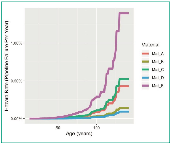
Figure 5: Hazard Rate for a Cox Proportional Hazards Model Showing the Effect of Pipe Material

Figure 5 shows the hazard rates from a Cox proportional hazards model showing the effect of pipe material. The graph shows the difference in hazard rate for each pipe material, with material Mat_E performing worse.

For a Cox proportional hazards model to be valid, the proportional hazards assumption must be confirmed. As the name suggests the hazard rates determined by the Cox model must be proportional. Methods to confirm the validity of the Cox proportional hazards assumption are Schoenfeld residuals, visual inspection of Kaplan-Meier survival curves, or visual inspection of log cumulative hazard curves.

Decision tree

Artificial intelligence algorithms such as decision trees and neural networks (deep learning) have been used for survival analysis. If the Cox proportional hazards assumption is not valid, or the Cox model is limited by low statistical power, or there are several predictors and a small sample size, then machine learning algorithms can be used for survival analysis. As research continues it can be expected that machine learning techniques will be utilised more in survival analysis.

The R package ‘LTRCtrees’ has been used in this paper to provide an example of machine learning for survival analysis because it can model the left truncated, right censored data considered in the pipes dataset. The ‘LTRCtrees’ package produces a decision tree which splits the data into homogenous sub-groups based on the covariates of interest. Figure 6 shows the decision tree produced by the ‘LTRCtrees’ package for the pipes dataset.

The decision tree produced can be used to predict the survival of pipelines.

Figure 6: Decision Tree Produced by the ‘LTRCtrees’ Package

Pipe dataset

A water utility typically has an asset register that contains the records of the pipelines in the water network. In addition, a database is maintained that records pipe bursts within the network. The dataset required for survival analysis of water pipelines is a combination of these two databases that contains all the mains in the system (including mains that have been decommissioned) joined to bursts recorded for each pipe.

The pipe dataset analysed for this report consists of 10,000 fictional pipe segments. Table 1 shows example data for five pipe segments which are representative of the data used for this analysis. In this paper pipe burst, pipe break and pipe failure all refer to a failure of a pipeline due to the structural condition of the pipe. In this report each pipe segment is referred interchangeably as a pipe, pipeline or main.

Each pipe segment has fields for pipe ID, episode, length of pipe segment (in metres), material, diameter (in mm) and status. The status field indicates if the pipe has failed (which is shown as a 1) or not failed (status of 0 – currently in service or it was retired before failure). The pipe material is referred to as Mat_A, Mat_B, etc. because this is a fictional database.

The burst year is recorded for each pipe segment that has failed. Pipe segments that have failed multiple times have a record for each burst. The episode number and pipe ID uniquely identify the record for each pipe segment.

It is usual to analyse multiple bursts for an individual pipe segment; however, consideration may be given to only analysing the first burst of each pipe. If a pipe is in very poor condition and repeatedly fails, this could increase the hazard rate for all pipes and lead to premature replacement.

Consideration should also be given to whether decommissioned mains that had many multiple breaks should be included in the analysis. Multiple breaks for poorly performing mains could bias the analysis and falsely indicate a higher hazard rate than if a poorly performing main is removed from the analysis.

Each pipe has a start age referring to the age of the pipe at the start of the record, which is either the age of construction, or the age of left truncation or left censoring. The stop age refers to the age of the pipe at the end of the record, either the age of failure or the age of right censoring or right truncation.

The start-stop format of Table 1 is called the counting process format which is useful for more complicated analysis such as recurrent events and time dependent variables. The data in Table 1 is recurrent data because one pipe segment can have multiple bursts. An example of a time dependent variable would be pressure for a pipe that was originally part of a high-pressure zone, and then became part of a lower pressure zone.

Censoring occurs when we know the event has or will occur, but we don’t know when. Records of pipes that have not failed by the date of observation or have been removed from service with no record of failure are considered right censored. Right censored records have a status value of 0.

Truncation refers to an absence of records of events, i.e. we don’t know if an event has occurred. The records for pipes constructed before burst data was collected are defined as truncated, and the start age of the pipe is taken to be the age of the pipe when the burst records start.

The pipes dataset used in this paper consists of 10,063 records for 10,000 pipe segments because there were 63 bursts recorded.

Table 1: Example Data

Other covariates that may be of interest that are not shown here include average system pressure, pressure during the burst, system pressure range, water supply zone, weather, cause of burst, type of burst, failure type, break location, ground condition, water temperature, corrosion protection, date and time of burst, land use, and depth of pipe.

Collection of this data is time consuming and some data may not be available for existing burst records (e.g. weather, pressure), however for future bursts it may be possible to collect this information automatically. It is expected that pressure will have a significant impact on pipeline survival rate.

Cause of bursts

Ensuring the accuracy of the burst record is essential for survival analysis. Accuracy refers not just to getting the facts right, but also to ensuring whether the burst was caused by the general pipe condition or operating environment and not due to an unrelated factor.

Pipe bursts that are really a connection failure, joint failure, fitting failure or accident do not represent a failure of the pipe due to its inherent condition and should be excluded from the analysis. This will allow the survival analysis to provide the best estimate of pipeline failure.

Failure of fittings, joints or connections should also be recorded, but analysed separately. If the connections on a main are failing it may be more cost effective to replace the connections on the main than replace the entire main. Similarly, if the lead joints on an old cast iron main are leaking, it may be more cost effective to repair the joints than replace the entire pipeline.

Variation in pipe length

For survival analysis it would be ideal for the length of each pipe segment to be the same because a long pipeline is more likely to burst than a short pipeline (for the same failure probability). However, the reality is that asset registers have pipes of varying length. Survival analysis can take account of this by including length as a covariate in the Cox proportional hazards model and determining the effect of length on survival rate.

If the Cox proportional hazards model shows length to be statistically significant to survival rate, then length can be included in the Cox model, or shorter pipes can be analysed separately to longer pipes.

Survival analysis as part of an asset management program

Development of a pipeline replacement program

The design life of a pipeline refers to a general estimate of the expected life of the main and is generally assumed to be 50-80 years.

The useful life of a pipeline is a realistic estimate of the time that a pipeline can meet standards of service.

The useful life could be defined as the age at which the pipe’s probability of failure (i.e. the hazard rate determined by survival analysis) reaches a predetermined value. The varying hazard rates shown in Figure 5 indicate that the useful life will be different for each pipe material – as expected.

The replacement date for a pipeline can be estimated by adding the useful life to the date of construction. When the replacement date for each pipe is determined these can be compiled in a pipeline replacement program. For the pipes dataset used in this report, the pipeline replacement program showing the estimated length of pipe to be replaced by year is shown in Figure 7 for a 0.05% probability of pipeline failure.

Potential uses of the pipeline replacement program within an asset management program are as follows:

1. Set or review service levels. The adopted probability of pipeline failure directly determines the useful life. The impact on the pipeline replacement program (and hence future expenditure) can be determined for different service standards (i.e. pipeline failure probabilities) and the service level set accordingly.
2. Allow planning for asset or non-asset solutions. By knowing the timing and cost of main replacements, a utility may be able to develop non-asset solutions, or alternatively identify that no non-asset solution is available.
3. Renew or dispose of assets. The pipeline replacement program provides a forecast replacement year for each pipe. Standard construction cost estimates can be used to prepare an estimate of pipeline replacement cost for each year based on the pipeline replacement program. This allows the utility to ensure it has the appropriate resources to replace the pipelines as required.

The major feature of Figure 7 is the large number of forecast replacements between 2063 and 2093. The average length of annual main replacement between 2019 and 2063 is 1,990m/year, and between 2063 and 2093 is 9,201m/yr.  The year 2063 may be a long time off but young engineers today may be in senior positions in 2063 when this becomes an issue. Planning for the large increase in annual pipeline replacement will need to be undertaken well before 2063.

Figure 7: Estimate of Annual Pipeline Replacement based on replacing mains when the probability of failure exceeds 0.05%

Cost benefit analysis

Survival analysis can assist the cost benefit analysis by providing a realistic estimate of the probability of pipeline failure. The probability of failure can be multiplied by the cost of pipeline repair plus the quantifiable economic cost of damage caused by the burst (e.g. damage to property, etc.) to provide an estimate of the economic cost of pipeline failure.

The expected economic cost of pipeline failure can be compared against the economic cost of pipeline replacement or rehabilitation to determine whether it is cost effective to replace a pipeline.

A risk matrix can be used to analyse non-economic costs to qualitatively compare the consequences of failure against the probability of failure. The risk matrix usually has the probability of an event on one axis and the consequence of an event on the second axis, and the risk being determined by the intersection of the two.

Survival analysis can inform the risk analysis by providing a defensible estimate of the probability of pipeline failure.

Unacceptable risks determined by the risk analysis must be mitigated by the project.

An important consideration in a cost benefit analysis is to look at actual burst records for the main being replaced. Survival analysis may indicate the main is part of a cohort of mains due to be replaced, but the replacement candidate may have no history of failures, and therefore deferral of pipe replacement may be justified.

For large diameter trunk mains that are very costly to replace, if the hazard rate for all trunk mains in a cohort indicates the pipe has reached its useful life, but an individual pipeline has better performance than other members of its cohort, deferral of main replacement may be justified for the better performing candidate.

For small diameter mains of a particular cohort, if the survival analysis indicates a high probability of failure (e.g. 100mm diameter AC mains older than 80 years), a utility may prefer to replace the entire cohort of these mains, rather than wait for each individual main to fail before replacement.

The utility will need to balance the desire to replace mains before they burst – and avoid the costs of pipeline bursts – against the cost of replacing mains that may not fail for some time. This decision will be a function of available resources and organisational priorities as well as survival analysis and cost benefit analysis.

Identify high risk areas

Analysis of bursts may show that a group of pipelines has a higher failure rate than predicted by the survival model. This could be because of construction techniques, pipe material, operating philosophy or other cause. Note, for this to be identified the appropriate covariates need to be included in the Cox proportional hazards model or decision tree model.

By investigating the reasons for variation in the probability of pipeline failure determined by the survival analysis, changes to operating or maintenance procedures may be identified that could improve pipeline survival. Examples of this could be lowering pressure, having a more stable pressure regime or the use of different pipe material.

Conclusion

Survival analysis can provide an estimate of the failure probability of water pipes based on burst history that can be used in asset management to provide a defensible mechanism to predict pipeline failure. The estimate of pipeline failure can be used to:

• Develop pipeline replacement programs,
• Determine the useful life of a pipeline,
• Inform a cost benefit analysis,
• Identify areas where the risk of pipe failure is higher, and
• Suggest effective methods to extend pipe life.

About the author

Gary Carlyle BE, MEngSci, GradDipIT | Gary Carlyle has worked in the water industry since 1989 in NSW and Queensland, and has worked for local government, state government and in the private sector. He also has experience in the IT industry.

References