Energy saving optimisation for water distribution networks

Abstract

Pump energy costs can be a major component of total operational expenditure for water utilities and it is a challenge to reduce pump energy costs while ensuring the continuous supply of high-quality water. Data61 and Sydney Water have worked collaboratively to develop intelligent network optimisation models to address the above challenge. Specifically, an energy saving optimisation model has been built to identify the optimal pump and valve operating schedules, so that peak-hour and shoulder-hour pumping is minimised and energy costs are reduced, while the required level of water quality performance is achieved. A simulation over three months demonstrated that a potential saving of around 15% in energy costs can be made with this approach.

Introduction

The Sydney Water Corporation supplies drinking water, wastewater, recycled water and stormwater services to more than five million customers in the Illawarra, Blue Mountains and Sydney metropolitan area. Pump energy costs can be a major component of operational expenditure for Sydney Water and other water utilities. For example, the pump energy costs for the Woronora Delivery System, accounts for 66% of the total operational expenditure of the system. Therefore, to minimise operational costs, it is important to reduce pump energy costs. On the other hand, water supply continuity also needs to be guaranteed.

This work addresses the above challenge by presenting a framework of energy saving optimisation in water distribution networks. More specifically, the objective is to optimise pump and valve operations, so that energy cost is minimised, water demand is met and reservoir operating window constraints are satisfied. In our previous work, analytics models for water demand forecasting, water quality modelling and chemical dosing optimisation have been developed (Mathews et al. 2017; Wang et al. 2018). This work focuses on the application of energy saving optimisation and more technical details of it can be found in our other publication (Zhao et al. 2019).

In particular, an optimisation model has been built based on water demand forecast to find the optimal operating schedule of pumps and valves for the next 24 hours starting at 7am every day. We have run a simulation over three months from December 2016 to February 2017 and have compared energy consumption and costs with historical data, which demonstrates that the optimisation model is effective in reducing energy consumption during peak and shoulder hours, resulting in a saving of around 15% in energy costs.

Business background

The Woronora delivery system

This work studies the Woronora Delivery System (see Figure 1), which includes 13 reservoir sites and supplies on average 80 ML (in summer months) of water per day to 210,000 customers in 30 separate pressure zones in the south of Sydney. Under normal operating conditions, the majority of raw water is supplied from the Woronora Dam. Due to data availability and quality, this study focuses on a subset of the system (six sites within the shaded rectangle – Figure 1). However, the methodology used in this work can be easily extended to the whole network when data become available for all sites.

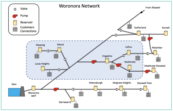
Figure 1: Woronora Water Supply Network

Energy cost

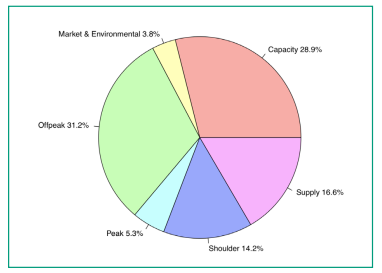
Figure 2: Components of Energy Costs

As shown in Figure 2, pump energy costs are composed of multiple components, including:

• demand charge (shown as peak, shoulder and off-peak in the figure), which is calculated with the amount of electricity used and the time of use,
• supply (or access) charge, which is of a fixed rate and charged by day or month,
• network capacity charge, which is calculated based on the maximum half-hourly consumption (KVA) that occurs in the peak tariff period (2pm-8pm on a working weekday) for the current month and has a rolling period of 12 months, and
• market and environmental charges, which are calculated with the total amount of electricity used.

The time of use for energy demand charges are

• peak: 2pm-8pm working weekdays,
• shoulder: 7am-2pm and 8pm-10pm working weekdays, and
• off-peak: all other times.

The figure shows that the network capacity charge and demand charge (including peak, shoulder and off-peak demand charges) account for around 80% of total energy costs. Therefore, to reduce energy costs, peak-hour and shoulder-hour pumping is to be reduced, because energy charge rates are higher in those hours and also because network capacity charge is calculated based on maximum half-hourly power readings during peak hours.

Datasets

Various data have been collected for the Woronora Delivery System, including:

• network topology data, including pipe characteristics and locations of control devices, such as flow meters, pumps and valves,
• customer water consumption data,
• monthly invoices for pumping stations,
• half-hourly energy consumptions and charges,
• pumping status and speed data – status and speed of pumps per 15 minutes,
• valve status data – status of valves per 15 minutes,
• flowmeter data – flow speed per 15 minutes, and
• reservoir data – reservoir water levels per 15 minutes.

We have also collected weather data from the Bureau of Meteorology, Australia, for water demand forecasting purposes.

Methodology

This application aims to optimise pump and valve  operations of the Woronora Delivery System (see Figure 1) utilising accurate water demand forecasts, so that energy costs are minimised, water demand is met, reservoir operating window constraints are satisfied and water quality performance is optimised. The input data include electricity consumption and cost, weather data, pumping and valve status, flowmeters and reservoir data.

Initially, at 7am every day, water demand is predicted with a Bayesian linear model, which forecasts the water demand of every reservoir supply zone in the next 24 hours. Thereafter, by taking input of initial reservoir levels, reservoir operating windows, pump operation and electricity tariffs, an optimisation model is built to minimise energy costs. A simulation over three months has been conducted for model validation.

Water demand forecasting

Figure 3: Water Demand Forecast – Engadine Zone

A prerequisite for optimising network operations, pumping schedules and reducing energy costs is accurately forecasting how much water will be used within different parts of the network. Water demand forecasting combines operational data and weather information about past and forecasted conditions and generates a prediction of short-term (24-36hr) future water demand. Specifically, factor analysis is firstly performed to identify important correlating factors, i.e. past flow, past and forecasted rainfall, past and forecasted temperatures, and a weekday/weekend flag.

A Bayesian probabilistic model is then employed to capture forecast uncertainty.

Figure 4: Water Demand Forecast – Engadine Zone
(incl. Demands from All Downstream Zones)

The result of water demand forecast at 7am for the Engadine zone is shown in Figure 3, where we can clearly see a high demand of water at 7am-11am and at 4pm-8pm. Figure 4 shows the demand of the same zone but including demands from all downstream zones, that is, those downstream reservoirs and reticulation zones that draw water from the Engadine reservoirs. There is a significant amount of water demand at 10pm-5am in Figure 4, which is caused by the filling of the downstream reservoirs during those off-peak hours. The forecast of cumulative water demand of a single site is shown in Figure 5a.

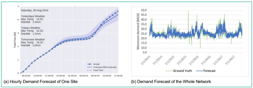
Figure 5: Results of Water Demand Forecast

The forecasting results have been evaluated by comparing the ground truth of historical data from 2 Jan 2014 to 31 Oct 2017. The Mean Absolute Percentage Error (MAPE) was used as the evaluation metric. Figure 5b demonstrates it can achieve reliable results except for some outliers in the historical records. The results of MAPE are 6.59% (summer), 4.33% (autumn), 4.07% (winter), 5.07% (spring) and 4.92% (overall).

The forecast error in summer is slightly higher than other seasons, likely because of more days with extreme weathers and total fire bans in summer. With an overall MAPE of 4.92%, this provides operational planners with accurate forecasts of water demand over operational windows, allowing more informed and timely trunk water operational decisions to be made.

Energy saving optimisation

Our energy saving optimisation model is shown in Figure 6 and an objective function is defined as below to model energy cost and constraints to reflect the relationship between water demand, water flow and reservoir water levels. However, if minimising energy cost for the next 24 hours only, the produced results would have minimum water levels at the end of the day, which would incur more energy cost in the next day. To mitigate the above issue, a penalty item is added to the objective function to make sure that the water levels at reservoirs at the end of the day would be close to the upper bounds. Therefore, the objective function is defined as

Obj ∶= EnergyCost + Penalty             (1)

where EnergyCost is the total electricity cost of all sites in the next 24 hours.

Figure 6: Energy Saving Optimisation Model

The optimisation of the above objective function is subject to 1) the relationship between reservoir levels, pumps and water demand, 2) reservoir operating windows, 3) the number of available pumps at every supply zone, and 4) the minimum daily water flow from the water filtration plant.

The relationship between reservoirs, pumps and water demand is defined as

V(t) = V(t-1) + P_in (t) – P_out (t) – D(t)                    (2)

where t is time (hour), V(t)  is reservoir level at the end of hour t, P_in (t) and P_out (t) are respectively the amount of water pumped into and out of the reservoir and D(t) is water demand from the corresponding zone.

Implementation

The above problem is formalised as an optimisation problem, which maximises or minimises an objective function by systematically choosing input values from within an allowed set and computing the value of the function. To meet a business requirement that the optimisation needs to run at 7am every day and produce an optimised pumping schedule within minutes, the optimisation problem is solved with Linear Programming.

It studies the case in which the objective function is linear and the constraints are specified using only linear equalities and inequalities and therefore the optimisation process is very fast.

The above optimisation was implemented with R (R Core Team 2018), a software environment for statistical computing and graphics, and the lpsymphony package (Kim et al. 2018), which adapts Symphony (Ralphs et al. 2017), an open-source mixed-integer linear programming (MILP) solver, for use in R. It was very fast and our experimental results showed that it took only 1.7 seconds on average for a 24-hour optimisation of six pumping stations.

Simulation and results

After modelling, a simulation was conducted over three months from 1 December 2016 to 28 February 2017 to validate the effectiveness of optimisation. At first, at 7am every day, optimisation ran to identify the optimised pump and valve  operating schedules for the next 24 hours. The reservoir levels were then updated based on historical demand and the optimised pumping schedule. This was followed up by going back to the first step to optimise for the next day. The above simulation process is illustrated in Figure 7.

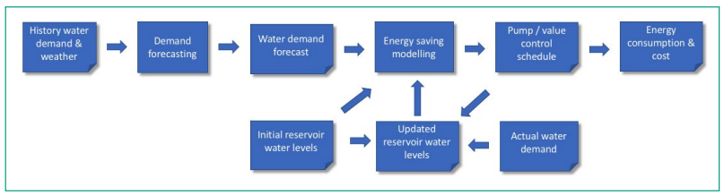
Figure 7: Simulation Process

Figure 8 shows the optimisation result for a pumping station on 6 February 2017, where the red solid line shows history and blue solid line optimised pumping schedules. The red dotted line shows history, the blue dotted line shows optimised reservoir levels, and the grey dotted lines shows lower and upper bounds of reservoir levels. With the optimised schedule, before 7am of every day, reservoirs are pumped with water close to their upper bounds, so that pumping during the following shoulder and peak hours can be reduced. Before 2pm, enough water is pumped into reservoirs to ensure that little or no pumping would be needed during the following peak hours. Figure 8 clearly shows that peak-hour pumping is reduced.

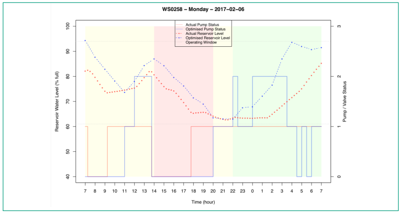
Figure 8: Optimised Pumping Schedule

We then compared the energy consumption and cost of the optimised pumping schedule with historical data. Figure 9a shows energy consumption of the pumping station during the three months, which also confirms that peak-hour and shoulder-hour pumping is significantly reduced. A comparison of energy costs shows that around 15% of energy costs can be saved with the optimisation model (Figure 9b).

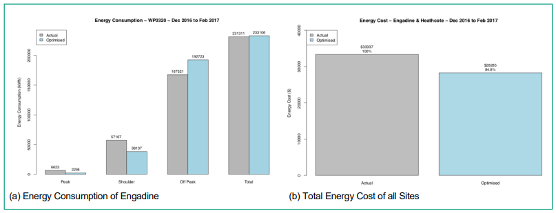
Figure 9: Simulation Results

With the optimised pumping schedule, most reservoirs have improved water quality, as shown in Figure 10.

Figure 10: Impact on Water Quality

From the simulation results, we identified the following observations. Some of them are consistent with existing domain knowledge and some provide new insights regarding pump scheduling. The observations are, to minimise energy costs:

• Off peak (22:00-7:00)
• Pumping as much water as possible
• Pumping water close to upper bound when off-peak ends at 7:00
• Morning and afternoon shoulder hours (7:00-14:00)
• Pumping water when needed
• At 14:00, reservoir should have enough water for demand up to 20:00, so that no pumping would be needed during the following peak hours.
• At 22:00, the water in the reservoir should be close to the lower limit, so that pumping in the previous morning shoulder hours is minimised.
• Peak hours (14:00-20:00)
• Avoiding any pumping if possible
• Evening shoulder hours (20:00-22:00)
• Pumping when the water level would become lower than the lower bound if no pumping

Conclusions and future work

The Woronora Delivery System has been studied and an analytics model has been developed that could considerably reduce the current energy costs while meeting water demand. A simulation over three months demonstrated that a reduction of 15% in energy costs could be achieved and that most reservoirs would have improved water quality.

In future work, optimisation on both energy saving and water quality will be integrated and performed iteratively. Moreover, the simulation needs to run for longer than a year, to further validate the impact on network capacity charge for the long term. Further  future work would be to reduce the number of times of starting/closing pumps and opening/closing valves, especially for large sites.

Acknowledgement

We’d like to thank the Sydney Water Corporation for their input of data and domain knowledge.

About the authors

Dr. Yanchang Zhao | Senior Research Scientist with Data61, CSIRO

Previously, he was a Data Analytics Lead with IBM (2017), a Senior Data Scientist with the Australian Government (2009-2016) and a Postdoctoral Research Fellow with UTS (2007-2009). He has authored/co-authored 60+ publications and is a Senior Member of the IEEE and a Steering Committee Member of the AusDM Conferences.

Dr. Bin Liang | Lecturer of Data Science at the University of Technology, Sydney (UTS)

Bin received his PhD degree from Charles Sturt University, Australia in 2016. Before joining UTS, he was a postdoctoral fellow in Data61-CSIRO. His research interests include data mining, computer vision, patter recognition, machine learning and survival analysis.

Dr. Shaobo Dang | Dr. Shaobo Dang is currently a postdoctoral research fellow on Autonomous Driving at SIAT, Chinese Academy of Science. Previously, he worked at Data61, CSIRO as a research engineer on data mining. He received his Ph.D. in Computer Science from the University of New South Wales in 2018. His research interests include data mining, traffic scenario awareness and safety evaluation.

Ronnie Taib | Ronnie Taib is a Principal Research Engineer with Data61, CSIRO. He has 20+ years’ experience in data analytics and user experience in organisations such as Alcatel Research and Motorola Labs and has a unique profile, mixing software and mechanical engineering skills, strong innovation (8 patents, 50 publications), and scientific research to design, manage and deliver high value-added technology projects.

Dr. Yang Wang | Dr. Yang Wang is an Associate Professor at the University of Technology, Sydney and a visiting Principal Researcher of Data61, CSIRO. He received his PhD degree in Computer Science from the National University of Singapore in 2004. His research interests include machine learning and information fusion techniques, and their applications to asset management, intelligent infrastructure, cognitive and emotive computing, and computer vision.

Professor Fang Chen | Professor Fang Chen is the Executive Director Data Science and Distinguished Professor at the University of Technology, Sydney (UTS). She has 300+ publications and 30 patents in 8 countries. She gained many recognitions such as the ITS Australia National Award (2014, 2015 & 2018) and the Australian Museum Eureka Prize for Excellence in Data Science (2018).

Dr George Mathews | Dr George Mathews is a Principal Data Scientist at QuantumBlack. Prior to this he was at Data61 and NICTA in Australia and BAE Systems in the United Kingdom. He obtained a PhD in Robotics from the University of Sydney in 2008.

Tin Hua | Tin Hua is an Operational Analyst with Sydney Water’s Operation and Analytics team, delivering water supply and wastewater services to over 5 million customers. He has 25 years’ experience in the water industry within the areas of operations, planning and data analytics.

Dammika Vitanage | Dammika Vitanage is the Asset Infrastructure Research Coordinator for Sydney Water. Graduating in 1980 with BSc (Hons) in Civil Engineering from the University of Peradeniya Sri Lanka, he now has around 39 years of water industry experience in asset management, operations, maintenance, and water quality, including more than 15 years in managing Research and Development.

Corinna Doolan | Corinna Doolan is a Customer Water Quality Manager with Sydney Water. She has been with Sydney Water for over 30 years, with extensive experience in drinking water quality management, operational strategies and project management, including planning and managing outcome driven research. Her research focussed on smart metering, end use studies, behavioural change, leakage management and intelligent network optimisation.

References

Vladislav Kim et al. 2018. lpsymphony: Symphony integer linear programming solver in R, projects.coin-or.org/SYMPHONY.

George Mathews, S. Lu, Zhidong Li, Ronnie Taib, Yang Wang, Fang Chen, Corinna Doolan, Robert Ius, D. Cash, Dammika Vitanage 2017. Data Driven Methods for Modelling and Optimising Chloramine Residuals. Ozwater 2017, Sydney, 16-18 May 2017.

R Core Team 2018: R: A Language and Environment for Statistical Computing. R Foundation for Statistical Computing, Vienna, Austria (2018), www.R-project.org.

Ted Ralphs, Ashutosh Mahajan, Stefan Vigerske, mgalati13, jpfasano, Aykut Bulut, & anhhz. (2017, January 17). coin-or/SYMPHONY: Version 5.6.16 (Version releases/5.6.16). Zenodo. doi.org/10.5281/zenodo.248734

Yang Wang, Zhidong Li, Yanchang Zhao, Ronnie Taib, Bin Liang, George Mathews, Fang Chen, Tin Hua, Robert Ius, Andrew Peters, Dammika Vitanage, Corinna Doolan 2018. Intelligent Network Optimisation Research Project – Final Report. CSIRO, Australia. December 2018.

Yanchang Zhao, Bing Liang, Yang Wang, Shaobo Dang, Ronnie Taib, Fang Chen, Tin Hua, Dammika Vitanage, and Corinna Doolan 2019. Optimising Pump Scheduling for Water Distribution Networks. In Proc. of the 32nd Australasian Joint Conference on Artificial Intelligence (AI 2019), Adelaide, Australia, 2-5 December 2019.