Data-driven water quality prediction in chloraminated systems

First published in Water e-Journal Vol 5 No 4 2020.

DOWNLOAD THE PAPER

Abstract

One critical aspect of overall water supply management is to monitor drinking water quality across the entire water delivery network. Compared with a model-based approach for water quality prediction, which simulates the real water quality decaying process using expert knowledge, a data-driven approach requires less business understanding.

This paper proposes a data-driven method that provides water quality prediction within the entire Woronora delivery system in Sydney. Specifically, the key factors relating to water quality are identified through factor analysis. A Bayesian parametric decay model is formulated using the key factors to predict water quality. To estimate the water travel time, which links the upstream (reservoir) data to the downstream (resident) data, the hydraulic system is employed to capture the topology of the delivery system. Moreover, the uncertainties of both data and the model are analysed to define the boundaries of prediction for better decision making.

The effectiveness of the proposed method has been validated using the data collected by online water quality analysers deployed in the distribution system. This work has established a successful initiative to improve the overall water supply management for the entire Woronora delivery system.

Introduction

Ensuring the delivery of clean and safe drinking water is a key objective for all water utilities. Within chloraminated networks, maintaining total chlorine levels is a key driver for the overall water quality. To investigate the technical and practical feasibility of applying innovative machine learning models to dynamically optimise the network operation to meet key performance indicators for water quality, Sydney Water, Veolia, and UTS Data Science Institute have studied the Woronora delivery system (see Figure 1) as a test use case. This is part of the 25 years of collaborative partnership of an innovative science and technology program between Sydney Water and Veolia for the Woronora and Illawarra Water Filtration Plants.

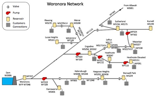
The Woronora delivery system includes 12 reservoir zones and supplies 80 ML of water per day to 210,000 customers in 42 separate pressure zones. Under normal operating conditions, the majority of the water is supplied from Woronora dam, with some water coming from Prospect Water Filtration Plant (WFP) via Allawah and into Sutherland reservoir.

The supply network is designed and operated to ensure three key objectives are met: 1) supply continuity, 2) water quality, and 3) pressure. The first ensures that water will remain available even in the event of a major disturbance such as the loss of power to pumps (minimum of eight hours of supply). The second ensures that the water is of acceptable quality and safe to consume. The third ensures there is sufficient pressure delivered to customers (minimum of 15m head). The system is operated to try to meet these requirements at minimum cost.

Continuity of supply and pressure requirements are generally met through defining minimum threshold levels for the reservoirs. These thresholds are to trigger the operation of pumps or inlet control valves.

A key aspect of meeting the water quality requirements is ensuring sufficient disinfection. Initial dosing of chlorine and ammonia occurs at the WFP, with secondary rechlorination at the reservoirs to top-up chlorine levels. Currently rechlorination is performed manually by adding chorine tablets to the reservoirs at specified intervals, e.g. twice per week. There are currently trials to move to an automatic dosing system that continuously regulates the reservoir chlorine levels. Sydney Water has an internal disinfection target of >0.60mg/L total chlorine for >90% of samples collected at the customers front tap.

The amount of chlorine added to the reservoirs is constrained by the amount of ammonia present in the water. The desired chlorine to ammonia ratio is 4:1. Above this, di- and tri- chloramine is formed which has an unpleasant smell and taste. Below this ratio, free ammonia is present and may be consumed by bacteria to produce nitrites and nitrates. This bacterial growth will also place a higher demand on chlorine.

The concentration of ammonia in a reservoir is generally dependent on the initial concentration of the water from the WFP, and how much has been consumed. This latter component is generally dependent on how much time has elapsed since initial dosing. The reservoir turnover targets are set to keep the residence time low. The residence time measures the average time that the water has remained in the reservoir and is dependent on how frequently the reservoir is refilled and the volume of water that is added in each refill cycle. The desired reservoir turnover is set by the system operators in consultation with the water quality team based on the ability to balance quantity and water quality.

Based on the Woronora delivery system, this work systematically studies the impact of network operations on water quality characterised by indicators such as total chlorine residual from the reservoir to customer taps. Historical network operation records, including reservoir levels, pump status, flows, pressures, dividing valve status, water demand, and water quality, are used as input data.

A prediction model for water quality has been built to provide quantitative predictions of total chlorine residual for the whole reticulation network downstream of reservoirs, for any target date included in historical records in different supply zones of the system. The water quality model aims to assist Sydney Water to meet the internal disinfection target of >0.60mg/L total chlorine for >90% of samples collected at the customers front tap.

Water quality modelling methodology

This section describes the quantitative model that links the upstream operational decisions and external influences on the water quality of the downstream customer connection points. The modelling is separated into reticulation network that extends from the reservoirs to the customers, and the trunk network that links the WFP to the downstream reservoirs. In modelling water quality within the reticulation network only the total chlorine residual, as the primary disinfectant, is considered.

In constructing the model, an initial factor analysis was performed to identify the key relationships between the available data and confirm assumptions regarding the causal influences. This follows the construction of a parametric Bayesian model.

Factor analysis

Here, an initial analysis is performed to identify the important system characteristics that may affect the downstream total chlorine residual. This is performed in a data-driven and non-parametric fashion that does not impose any assumptions on the structure of the relationships. The objective is to identify the dependencies that may exist in the data, without making upfront assumptions on what chemical or physical processes are at work.

An integrated dataset has been assembled by combining sample data for the reservoirs and compliance tap sites, along with level sensors and water quality analysers at the reservoir sites. The dataset allows the relationships between the total chlorine at the tap sites and reservoir information regarding total chlorine residual, water temperature, pH balance, turbidity, ammonia concentration, and reservoir levels.

To detect the critical variables, or factors, that can help explain or predict the downstream total chlorine residual, an exploratory regression analysis has been performed. This uses a non-linear and non-parametric regression model based on the Random Forest algorithm (Breiman, 2001).

A recursive analysis is performed where, starting with all factors, each factor is considered in turn and the factor that produces the smallest reduction in predictive error is removed. This recursive elimination is repeated until all features have been removed. This enables the most important predictive factors to be identified, with the results depicted in Figure 2. The baseline error represents the average error in the mean total chlorine residual and characterises inherent variability in the data. This represents the removal of all factors.

The analysis shows that reservoir total chlorine and temperature capture over 90% of the variability in the downstream total chlorine that is explainable by the data (and about 50% of the total variability). Reservoir level, chlorine to ammonia ratio, and pH have a much smaller effect. Turbidity provides virtually no additional information. This analysis confirms the importance of the initial total chlorine residual at the reservoir, and the effect that temperature has on the decay properties.

Total chlorine decay modelling

With the two critical factors of reservoir total chlorine and temperature identified, a causal parametric model is now explored. Analytical models for free and total chlorine dynamics often consider a first order decay model, with extensions that include multiple reactants, and separate bulk and wall decay processes (Fisher, 2012; Monteiro, 2014; Nejjari, 2014). For instance, a simple first order model, with decay rate or decay coefficient denoted by k is defined by the equation

 

Integrating this produces the exponential decay curve C=C_0 exp⁡(-kτ) where C_0 is the initial total chlorine residual, and τ is the elapsed time.

Temperature dependence is often included through an explicit functional dependency such as a simple linear, exponential or Arrhenius’ equation (Monteiro, 2014). For example, a linear model for the decay rate, where T denotes the water temperature, defines the decay rate as

The analysis has shown that chlorine decay rates, as measured in a controlled laboratory environment, exhibit significant variability. This is unlikely due to chlorine measurement errors alone and the high degree of variability may or may not be driven by temperature changes. The observed relationship between initial decay rates and the initial water temperature shows a very slight upward trend with temperature.

Furthermore, it is expected that the decay characteristics within the network will show even higher variability and a full statistical analysis will be needed to determine the influence between temperature, measurement errors and other potential influences.

Statistical modelling of decay dynamics

In what follows, the parametric Equations (1) and (2) will be used to define the underlying chlorine dynamics, and the in situ operational data will be used to characterise the parameter variability and uncertainty. This departs from all known past work that uses an analytical decay model to predict downstream chlorine residuals.

These methods typically assume that the free parameters that govern the dynamics (e.g. k_0 and k_1) are unknown but time invariant constants that are selected based on some calibration process, for example, to minimise the squared difference between model predicted chlorine concentrations and those measured in the network (Nejjari, 2014). This type of calibration process not only assumes that the parameters are constant, but that the time the water takes to travel through the system is also known precisely. This requires, for instance, all the network flows and customer demands to be known. These assumptions are unlikely to hold in real systems.

It is noted that the first order decay model with simple linear temperature dependence represents a relatively simple model and more complex extensions could be considered. However, as the model becomes more complex, with more free parameters, it may become better at reproducing the past observations (i.e. the training or calibration data).

However, at the same time it may become poorer at predicting new measurements at other locations in the network or time in the future. This is the well-known problem of overfitting. Here, the use of a simple model (total chlorine decay modelling) developed based on factor analysis insights (factor analysis) is expected to avoid the issues with overfitting, while introducing some additional bias. Although this is not ideal, the additional bias is at least partially observable in the training data and can be characterised in a data-driven fashion.

Thus, the critical objective here is to construct a statistical model that can quantify the uncertainty and inherent variability in the system and allow predictions to be generated for new sites with the network.

Travel time estimation methodology

A critical input to the parametric decay model is knowing the time it takes water to travel through the network, for instance from a chlorine analyser at a reservoir outlet to a downstream customer connection point. It is noted that the travel time cannot be measured directly and must be estimated indirectly.

To do so, each zone is considered separately combining the available flow data, as illustrated in Figure 3. The total incoming and outgoing flows of each zone can be estimated by considering the data from the flowmeters and reservoir level sensors. These are available at a high frequency of one measurement per 15-minute period. In addition to this, the meter data of individual customers provide detailed spatial data on the outflows on the network, but at a very low temporal resolution of once per month (interpolated from quarterly meter readings).

To estimate the time it takes water to travel from, for example, the upstream reservoir to a location in the network, an assumption must be made on the temporal variation in the demand at the customer locations. Here, it is assumed that all the customers consume a fixed proportion of the total water that is consumed within the zone.

For example, if during a peak demand time the total consumption within the zone is twice the average, it is assumed that all customers will be consuming twice their average demand. This assumption provides a way to use the high frequency flowmeter data to interpolate temporally the individual customer demand. It is noted that this does not differentiate between residential, commercial, or industrial customers that may consume water at different times during the day. Such an extension could be considered in the future.

It is acknowledged that this assumption on how water is used by customers is an explicit simplification and any network flows that are estimated with this assumption will be incorrect. Nevertheless, it provides a good starting point for estimating the travel time between two points in the network. In what follows, an additional error model will be constructed to reflect the approximate nature of the hydraulic model.

The travel time estimation can be performed using standard hydraulic flow simulators by first computing the flow rates on each pipe segment, followed by a path tracing algorithm to compute the total travel time. Based on the available data from flowmeters and water consumption by customers, we have studied 12 reservoir zones in the delivery network as shown in Figure 4. The travel time for each reservoir zone is estimated and shown in Table 1.

Decay model

To incorporate the known variability in decay rates and the travel time estimation errors, a full statistical decay model is now defined. Firstly, consider a customer connection point at a network location. The estimated travel time between a given upstream reservoir and location s at time t is dependent on the network topology and the assumed demands for all customers in the network. This is computed through a standard deterministic hydraulic simulation with the assumptions outlined above and is denoted τ ̂_(t,s) (the hat denotes an estimated value). For the networks under consideration this typically takes values up to 48 hours. The upstream total chlorine residual denoted C_(t,s)^u and represents the delayed total chlorine measurements at the upstream reservoir site, for instance, provided by the chlorine analysers;

C_(t,s)^u=C_Reservoir (t-τ ̂_(t,s)).

Where C_Reservoir (t) represents the time series of measurements made by the online chlorine analyser at the reservoir. Furthermore, let the measured water temperature of the upstream reservoir be denoted by T_(t,s)^u.

The predictions of interest are the total chlorine residual at downstream locations and will be denoted be C_(t,s). The compliance measurements represent observations of this for a limited set of locations and times, (t,s)∈M_comp.

The first order temperature dependent decay model, specified in Equation (1) and (2), provides a link between the operational data that comprise the upstream reservoir total chlorine residual, water temperature, and estimated travel time between the reservoir and the downstream location. This set of data is denoted by
d_(t,s)={ τ ̂_(t,s),C_(t,s)^u,T_(t,s)^u}.

Written explicitly, the model equation is

C_(t,s)=C_(t,s)^u exp⁡(-τ ̂_(t,s) (k_0+k_1 T_(t,s)^u)). (3)

This can be written compactly as C_(t,s)=f(d_(t,s),θ) where θ incorporates the decay parameters k_0,k_1.

As highlighted previously, the above decay model makes approximations in multiple areas including:

The actual time it takes water to travel through the network may be larger or smaller than the estimated value τ ̂_(t,s).

The measurements of temperature, and total chlorine, are all subject to measurement errors.

The actual decay rate is not only dependent on temperature and may change due to other unmodelled effects.

To properly represent the relationship between the data, parameters and the predictions, all these unknown errors should be considered. It is noted that this is far from straight-forward as even the likely magnitude of the errors is unknown and it is not often practical to perform a targeted test (e.g. a bench top test, tracer test) to estimate them in a reliable fashion.

The proposed probabilistic modelling approach enables all these error characteristics to be estimated in situ using only the available real-time operational and sparse compliance data. To define this model, consider the deterministic model that links the real-time operational data to the downstream total chlorine residual in (3). This is extended to incorporate errors in the travel time and decay rates with an unknown, but positive, scale factor ξ. The unknown measurements errors and other unmodelled effects are represented with an additive factor ε. These errors may be different at each time and location in the network depending on environmental conditions. The extended model equation becomes

C_(t,s)=C_(t,s)^u exp⁡(-ξ_(t,s) τ ̂_(t,s) (k_0+k_1 T_(t,s)^u))+ε_(t,s). (4)

The additive errors are expected to be centred on 0 and may be positive or negative. It is assumed that for any s and t, the errors are independently and identically distributed according a Gaussian distribution with median of 0 and unknown variance, denoted by σ_ε^2. The scale errors are expected to be centred on 1, and must be strictly positive. It is assumed that these errors are independently and identically distributed according to a log-Gaussian distribution with median of 1 and unknown variance, denoted by σ_ξ^2. This distribution is chosen such that the probability that ξ lies in the interval [1,a] is the same as the probability it lies in the interval [□(1/a),1] for any a≥1.

The unknown terms in Equation (4) are separated into decay parameters θ={k_0,k_1}, error terms e={ξ_(t,s),ε_(t,s)}, and error strength parameters ϕ={σ_ε,σ_ξ} that define the probability distribution for the error terms e.

Model training

To enable new predictions to be made for downstream sites at new locations, it is required to infer the decay parameter k. This is performed using the measured total chlorine residuals obtained from the compliance sites. This inference is solved using the least squares regression by curve fitting.

To enable new predictions to be made for downstream sites, either at new locations and/or times, it is required to infer the decay parameters θ={k_0,k_1} and error strength parameters ϕ={σ_ε,σ_ξ}. This is performed using the measured total chlorine residuals obtained from the compliance sites.

A full Bayesian inference procedure is performed to generate a probability distribution over the parameters θ,ϕ given the available operational and compliance data, and loosely constraining priors for θ and ϕ. The priors are defined via a set of hyperparameters that are selected based on expert knowledge of expected decay rates and other information. Example decay curves, based only on these loosely constraining priors, are depicted in Figure 5.

A separate model is constructed for each reservoir zone, based on the available downstream compliance measurements C_(t,s), and the corresponding travel time, upstream chlorine and temperature information, denoted by d_(t,s). The training dataset for a given reservoir is denoted by D={C_(t,s),d_(t,s):(t,s)∈M_comp}, where M_comp denotes the set of times and tap locations within the network where the past compliance measurements have been made.

The posterior distribution of the parameters  is proportional to the prior and the likelihood

p(θ,ϕ│D)∝p(θ,ϕ)p(D|θ,ϕ)

This inference problem is solved using the hybrid Monte Carlo sampling scheme. The median parameter estimates for the four variables are plotted in Figure 6 for each zone. The complex set of pairwise plots that show the uncertainty in the parameter estimates, as well as the correlations between parameters, is displayed in Figure 7.

References

Breiman, L. (2001). Random forests. Machine learning, 45(1), 5-32.
Fisher, I., Kastl, G., & Sathasivan, A. (2012). A suitable model of combined effects of temperature and initial condition on chlorine bulk decay in water distribution systems. Water research, 46(10), 3293-3303.
Monteiro, L., Figueiredo, D., Dias, S., Freitas, R., Covas, D., Menaia, J., & Coelho, S. T. (2014). Modeling of chlorine decay in drinking water supply systems using EPANET MSX.
Nejjari, F., Puig, V., Pérez, R., Quevedo, J., Cugueró, M. A., Sanz, G., & Mirats, J. M. (2014). Chlorine decay model calibration and comparison: application to a real water network. Procedia Engineering, 70, 1221-1230.