Cost-effective monitoring of impacts on seagrass

Abstract

Seagrass meadows in Australia are at risk from a range of anthropogenic stresses including effluent discharges from wastewater treatment plants, brine discharges from desalination plants, industrial discharges from refineries, power stations, hydrogen hubs, dredging for port activities, marinas, transfer ports for offshore wind turbines, as well as runoff from urban areas. There is continuing urban growth in many of the catchments draining to areas with extensive seagrass meadows.

Monitoring seagrass is challenging: Seagrass meadows are naturally patchy and the patches vary from season to season and year to year. The area of seagrass meadows changes with long-term patterns in rainfall and runoff and on a smaller scale due to predation and disease.   

Aerial images from satellites are an economical method to monitor the general extent of seagrass, but high-quality images are uncommon, as clouds, rain and turbidity make it difficult to see the meadows clearly with the edges and holes difficult to discern.

Underwater camera photographs, particularly if taken on lines in a grid, provide much more information. Reliable estimates can be made of seagrass species distribution and density, as well as percentage macroalgae and epiphyte cover from underwater photographs. Although costly, this is the premier method to make a good seagrass inventory.  
Diver measurements of morphological characteristics are precise, but only a very small area can be surveyed within a reasonable budget. 

A new method using drone photographs to determine seagrass cover and extent is presented in this paper, with an example from Corio Bay. The drone method offers a cost-effective procedure for long-term monitoring of seagrass conditions by the water industry.

Introduction

Seagrass grows in shallow water where there is sufficient light to allow growth of the plants.  Australia has approximately 51,000 km2 of seagrass meadows in shallow subtidal and intertidal environments (MESA, 2025). The meadows are generally found in estuaries and sheltered bays where there are weak ocean currents and limited wave action (and thus limited sediment erosion and movement).

Seagrass is an ecologically significant marine habitat that provides food and shelter for many marine organisms (Orth et al 2006). Swans and sea urchins feed directly on seagrass while other animals graze on epiphytes growing on the stems and leaves.  Seahorses and small fish shelter among the seagrass leaves. Seagrass detritus provides food for benthic fauna and these in turn provide food for fish, crustaceans, birds and waterfowl (Blake and Ball, 2001).  Seagrass meadows provide habitat for fish including nursery areas for juveniles.  

Seagrass meadows in Australia are at risk from a range of anthropogenic stresses.  In Port Phillip Bay, VIC, seagrass meadows are stressed by effluent discharge from the Werribee, Altona and, occasionally Carrum wastewater treatment plants; brine discharge from the Altona desalination plant; cooling water discharge from the Newport power station; dredging for port activities and marinas; as well as runoff from the urban areas of Melbourne.  

In Boston Bay, SA, seagrass meadows are stressed by effluent discharge from the Port Lincoln wastewater treatment plant; the future brine discharge from the Port Lincoln desalination plant; dredging for marinas and runoff from urban areas.  

In Cockburn Sound, WA, seagrass meadows are stressed by effluent discharge from the Point Peron wastewater treatment plant; brine discharge from the Kwinana desalination plant; cooling water discharge from the Kwinana power station; industrial and cooling water discharges from a refinery, fertiliser, alumina, titanium and chemicals industries; dredging for an expanded port; ship construction and naval activities.

In Moreton Bay, QLD, seagrass meadows are stressed by effluent discharge from the Luggage Point wastewater treatment plant; dredging for the port; industrial discharges coming down the Brisbane River and the extensive reclamation for the Port of Brisbane.

In Corio Bay, VIC, seagrass meadows are stressed by regular dredging for the existing port and by discharges from shipping and the refinery. Stresses are likely to increase as there are proposals for an LNG import terminal, hydrogen generation, a terminal to receive, store and ship offshore wind turbines and for major urban development in the catchment.

There have been significant losses in seagrass meadows in Australia, with an estimated total loss of  300,000 ha (Walker and McComb, 1992). This loss is attributed to a combination of factors but mostly to nutrient discharges (Cockburn Sound, WA; Oyster Harbour, WA); sediments (Western Port Bay, VIC) or high nutrient and sediment inputs (Adelaide, SA).  

The 60% loss of seagrass in Adelaide was attributed to wastewater effluent and sludge discharge, and stormwater inputs along the coast (EPA SA, 1998). The 79% loss of seagrass in Cockburn Sound was attributed to the discharge of nutrients (Cambridge and McComb, 1984). The causes of the 85% loss of seagrass in Western Bay are not fully understood but are attributed to sediment inputs (EPA VIC Bulletin 588, 1997). The 20% loss of seagrass in Moreton Bay is attributed to sediment and nutrient inputs from wastewater treatment plants and runoff (BMT, 2023).

From these examples, it is apparent that the water industry has a significant influence on seagrass health in Australia and, therefore, an interest in monitoring seagrass health in a cost-effective way.

Methods for monitoring seagrass

There are four general methods to monitor seagrass health:

1. Analysis of aerial images or photographs;
2. Underwater camera photographs from a boat or remotely-operated underwater vehicle;
3. Diver measurement of morphological characteristics; and
4. Integrated photographs obtained using a low-flying drone.

Aerial images provide a good indication of the total area of seagrass in the region, but with lower accuracy in deeper water where visibility is limited and seagrass plants are more sparse. The extent of subtidal seagrass can be mapped in the images using GIS polygons to identify the boundaries of medium to dense seagrass. This method provides a measure of overall seagrass extent, but not the density of seagrass cover.

The advantage of aerial images is that large areas of seagrass can be surveyed quickly. The main disadvantages are that clouds, waves and turbidity in the water column limit the ability to distinguish seagrass and the classification is generally presence/absence, with limited ability to discern changes in seagrass density or light, patchy seagrass areas. Unless special aerial surveys are undertaken, good quality and readily available images may occur only once a year. Also, macroalgae (such as Caulerpa) can cover seagrass and ground-truthing surveys are required to check marine vegetation mapped from high-altitude aerial images.

Underwater towed camera photographs provide a very good indication of seagrass species and cover along the camera track, as well as epiphyte density and macroalgae species and cover. The angle of the camera can be adjusted to provide a good image of the seabed in both shallow and deep water. The camera position is logged within +/- 2 m using GPS and a depth sounder. This is the premier method for monitoring seagrass, particularly when a grid of tracks is used. 

A CCTV on the vessel towing the camera shows the images being recorded and personnel in the vessel can record observations at the time of viewing, while images are saved for subsequent evaluation and analysis. A towed camera can be used effectively in water depths of less than 2 m to more than 50 m.  

The advantages of underwater photographs are that detailed images of seagrass, as well as associated biota including epiphytes, macroalgae and large marine pests, can be identified and the images can be used to classify seagrass density (or cover) as well as the density of other marine species. The disadvantage is that images cover only a small area (0.8 to 1 m2) and need to be collected using a vessel travelling at a low speed (about 2 km/hr). The seagrass is sampled in strips and it is seldom feasible to cover the entire seabed in a large area. It is also not feasible to survey in shallow water which is often where high density seagrass occurs. 

Diver surveys collect a large amount of information on seagrass in a small area. The information is typically stems per m2 and abundance and type of epiphytes. Stems can be harvested and further measurements can be made (length and thickness of stems, length of stems, length of leaves, number of leaves per stem, dry weight of plant). The advantage of diver surveys is that they can be conducted over the full depth range of seagrass and that detailed data on morphological characteristics are obtained.  
The disadvantage is that only very small areas are sampled (typically 5 quadrats of 0.25 by 0.25 m, or 10 quadrats of 0.2 by 0.2 m) so the area surveyed is only 0.03 to 0.04 m2 for a considerable diver input. 

Drone photographs provide good data on seagrass cover in the intertidal zone and shallow seawater.  An advantage is that drone photographs have high resolution and more detail than aerial images, as the drone is only 40 m above the water, and excellent position fixing. The quadrats used in the analysis of drone images can be large – 2 m by 2 m, as illustrated in the example below, so that large areas of seagrass can be monitored with spatial and temporal variations in seagrass measured and taken into account in calculating percentage seagrass cover.

Drone photography is much cheaper than an underwater camera outfit or a diving team and hence is suitable for long-term regular monitoring.  

Determination of seagrass cover

Extra information on seagrass condition can be obtained from underwater images and drone images. The most useful parameter is seagrass cover – the percentage of the seabed covered with seagrass as this relates directly to the productivity of the seagrass meadow. 

Seagrass is naturally patchy. Seagrass cover is a metric that takes account of this variability and establishes the area of seagrass that is actively photosynthesising. The method used to convert the appearance of seagrass in the images to percentage seagrass cover can be made using the scale developed by Blake and Ball (2001) as summarised in Table 1.   

Table 1: Classifying percentage seagrass cover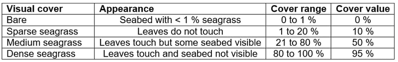

The same seagrass classification categories (dense/medium/sparse/bare) were used in the Victorian Multi-regional Seagrass Health Assessment 2004–2007 (Ball et al, 2010) to map seagrass in various areas of Port Phillip Bay and Corio Bay.   

The procedure has since been used in over 20 seagrass studies for various water quality investigations in Port Phillip Bay including the Baywide Seagrass Monitoring Program during a major channel dredging program (Hirst et al, 2015).

A sensitivity analysis of the cover classification was undertaken with the resulting percentage cover being calculated within 1 % with repeated classification with or without the medium range being sub-divided. A computer program incorporating AI can be used to develop a more accurate percentage seagrass cover from drone images.

Measurement of seagrass cover from drone images

In Corio Bay, the most dense seagrass meadows are in shallow water from low tide to 2.5 m depth. Monitoring by drone imagery was adopted because it was not feasible to use an underwater camera towed by a boat in the shallow water. The results are compared to seagrass monitoring using an underwater camera at 3 m depth and to seagrass extent from aerial images.  

An example of the application of the drone method is presented later where it is used to assess the effects of a cooling water plume on seagrass.

The method adopted for monitoring seagrass cover from drone images involves:

• Taking images from a low-level drone with a high resolution camera flying on a grid;
• Integrating the images using a GIS program to obtain a complete rectified image of the study area;
• Defining sampling quadrats of 2 m by 2 m area along depth transects at m intervals;
• Applying the classification scale shown in Table 1 to determine the average seagrass cover in each quadrat.
• Combining the results for quadrats to determine the percentage seagrass cover in the study area.

The transects were typically 400 m to 600 m long, so seagrass meadows over 2 km were surveyed. The quadrats were each 4 m² in area at 15 m spacing, so seagrass in a total area of about 100 m² was surveyed on each transect. This is substantially larger than the 0.4 m² achieved in a diver survey. The spacing of quadrats can be refined to suit the study.

Figure 1 shows examples of the seagrass cover results on 30 quadrats along two 600  m long transects at different depths. The upper transect is just below low tide and shows a mixture of empty patches (short orange columns); sparse seagrass (short light green columns); moderate seagrass (medium green columns); and dense seagrass (tall dark green columns).  Seagrass cover on this transect was 75 %.

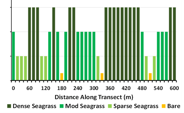
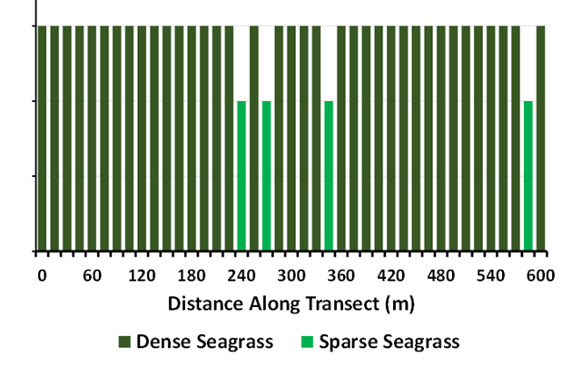
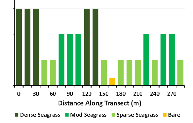
Figure 1: Examples of seagrass cover data

The middle transect is at 1.8 m depth and shows mostly dense seagrass cover with four patches of moderate seagrass. Seagrass cover on the second transect was 89 %.

The lower transect is a shorter transect along the coast at 0.8 m depth and shows mostly moderate seagrass cover with patches of sparse and dense seagrass. Seagrass cover on the third transect was 43 %.

Analysis of the drone images gave an excellent record of the distribution of seagrass on a fine scale in Corio Bay. Over the whole of northern Corio Bay, the drone images showed the average seagrass cover was 71 % (from zero to 2 m depth). An interpretation of this result is that in the shallow waters of Corio Bay, seagrass covers 71 % of the seabed and the other 29 % is bare seabed or open patches in the meadows. 

Monitoring seagrass by underwater images

Seagrass conditions in Corio Bay were recorded using a towed underwater camera with a 3 km long longshore transect on the 3 m depth contour and regular onshore-offshore transects at about 200 m spacing. A total of 11,600 underwater camera images were obtained over a total length of 10.5 km.  The underwater camera images of seagrass in Corio Bay were assessed for seagrass cover and for the abundance of macroalgae, microphyto-benthos, seabed character and bioturbators. Seagrass cover was calculated using the same procedure as for the drone images.  

Seagrass in the northern Corio Bay area can be classified into three zones: 

1. Nearshore - H. nigricaulis mixed with (N. muelleri) – 14 ha;
2. Shallow water - Dense H. nigricaulis mixed with small patches of Althenia – 43 ha;
3. Deeper water - H. nigricaulis mixed with Halophila – 120 ha, being predominantly H. nigricaulis closer to shore and mostly Halophila in deeper water.

Applying the classification scale shown in Table 1, the overall seagrass cover from the towed camera images was 64 %. This is slightly lower than the cover calculated from the drone images of  71 % as seagrass cover and density are lower at greater depths.

Seagrass cover from aerial images

A further check on seagrass cover measurement was made using aerial images of Corio Bay.  High-quality aerial images of Corio Bay were sought from the 15-year period 2010 to 2025.  Only seven images were found to be suitable, as the others had problems with cloud cover, reflectance of the sun, elevated turbidity in the water column or high tide.

The extent of subtidal seagrass was mapped in the images using GIS polygons to identify the boundaries of medium to dense seagrass boundaries in the study. This method provides a measure of overall seagrass extent, but not the density of seagrass cover.

Figure 2 shows the variation in seagrass cover in Corio Bay VIC for the years 2011 to 2023, from high-quality aerial images. The cover (percentage of seabed with seagrass) varied from 50 % to 76 % with an average of 63 %. 

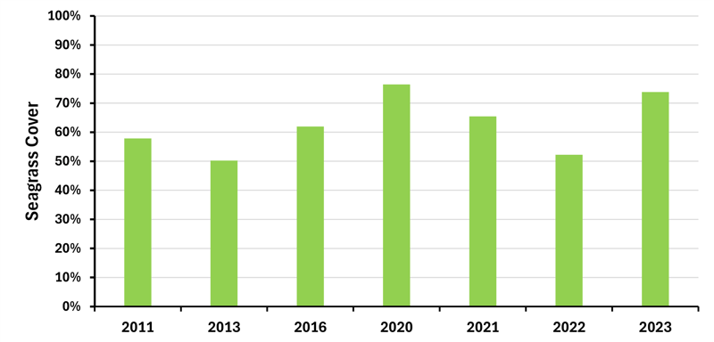
Figure 2: Seagrass area in Corio Bay from aerial images

The average seagrass cover from the aerial images of 63 % (from zero to 5 m depth) is slightly below the results from the underwater camera. An interpretation of the result from the aerial images is that seagrass covers an average of 63 % of the seabed and the other 37 % is bare seabed or open patches in the meadows.

Seagrass cover as an indicator

Vegetation cover (density and area) is a metric used in a wide range of marine and terrestrial environments for management, assessment and scientific applications. Seagrass cover has been used in several previous studies of seagrass in Corio Bay and Port Phillip Bay (CSIRO 1996; MSE 2006; Ball et al 2014). Eigenraam et al (2016) used hectares of seagrass cover (with other ecosystem descriptors) in Corio Bay to assess environmental services and values. 

In adjacent Port Phillip Bay, seagrass cover was measured in 2011-2013 from aerial images of 30 sites with areas of 30 ha to 100 ha and a series of morphological parameters (shoot biomass, rhizome biomass, shoot/rhizome ratio, maximum shoot length, seed density) were measured in ten plots of 4 m² (total area of 40 m²). The plots were sampled twice a year (Jenkins et al 2015).

From a statistical analysis of the measured parameters, Hirst et al. (2012) concluded that percentage seagrass cover is the most useful proxy for seagrass health because it is strongly correlated with the other major parameters, as reflected in a Principal Component Analysis.  Seagrass cover is the simplest variable to measure in the field and provides the most data for a given level of expenditure – seagrass cover can be determined in 100 ha for a lower cost than morphological parameters in only 40 m² (or 0.04 ha). In summary, seagrass cover is considered the most cost-effective seagrass parameter to measure.

Variations in seagrass cover from year to year

As illustrated in Figure 1, seagrass meadows are naturally patchy and variable over time. Thus, the monitoring technique needs to recognize and record this spatial and temporal variation. The example from Corio Bay in Figure 2 shows that aerial images record the year to year variation in total cover, while the underwater camera and drone images methods record the spatial variation in the seagrass meadows as well as the year to year variation.

Long term monitoring of seagrass is required because seagrass is so variable. Even the stable and persistent seagrass meadows in Corio Bay show a +/- 12 % variation in area from year to year (calculated as the standard deviation of values in Figure 1).

Seagrass on Moreton Bay has been monitored annually for approximately 20 years by the Port of Brisbane at a site next to the reclamation for the Port of Brisbane and other reference sites, including Manly 2 km to the east (Port of Brisbane website, May 2025). In each area, seagrass is recorded using a static underwater camera at points on a 500 m grid extending approximately 6 km by 2.5 km. There are generally five different species of seagrass in the sampling areas and seagrass is classified as “light” if < 10 % cover; “medium” if 10-50 % cover; and “dense” if > 50 % cover. Most sites are bare or light cover, with a small proportion having medium cover.

There were periods of significant increase in seagrass cover and extent in 2010 and 2017, with declines in 2011, 2013  and 2022, which corresponded to high rainfall and runoff. A secondary factor is the seasonal variation in water quality with lower turbidity in June to September when Halophila ovalis extends further offshore into deeper water (BMT 2023).

The Port of Brisbane reports do not provide data on overall seagrass cover but do provide the percentage cover of different species and the percentage of grid points with any seagrass.  However, the data can be transformed to show the approximate seagrass cover in the Moreton Bay sites.

Figure 3 shows the variation in seagrass cover in two sites in Moreton Bay over the last six years (data from Port of Brisbane website, 2025). Typically, seagrass cover is in the range of 10 to 15 % of the seabed in the surveyed sites, with a similar variation at Fishermans Island and the reference site at Manly. These changes are likely to be associated with variation in climatic conditions (particularly rainfall and wind patterns, which influence water turbidity). Seagrass in Moreton Bay is mostly sparser than seagrass in Corio Bay.

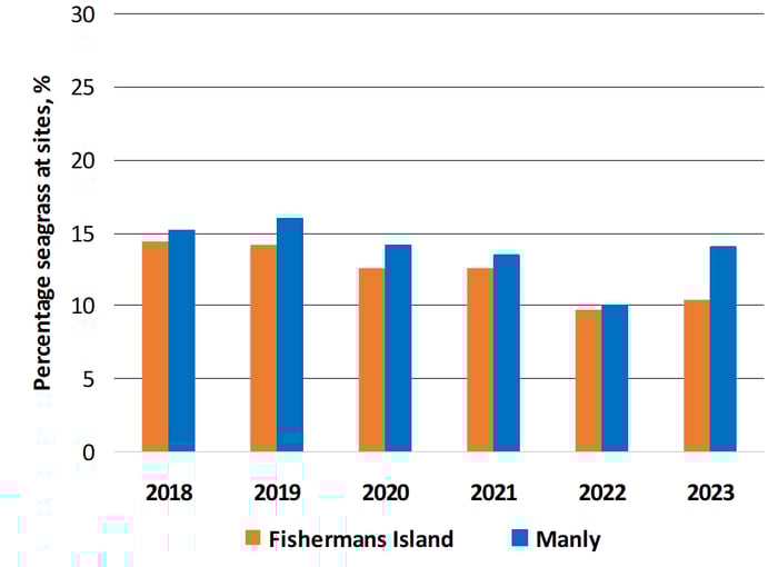Figure 3: Seagrass cover in Moreton Bay from spot underwater images

In Cockburn Sound, seagrass is monitored annually at up to 27 sites, including five reference sites (Cockburn Sound Management Council, 2021). Although measurements are made of various metrics, including stem height and lower depth limit, the main metric used to determine seagrass condition in Cockburn Sound is shoot density (number of seagrass stems per m²).  There are 1 %, 5 % and 20 % limits for seagrass (Posidonia sinuosa) shoot density based on rolling 4-year values measured at reference sites. The limits decrease with depth and are typically about 700 shoots/m² for sites at 2 m depth.

Divers count the shoots in quadrats of 0.2 m by 0.2 m (area of 0.04 m²) with 10 to 24 quadrats per transect. Typically an area of 1 m² is monitored along a single line. 

Figure 4 shows an example of the results for two transects on Cockburn Sound (data from Cockburn Sound Management Council, 2024). The number of shoots per m² varies from year to year, between 500 and 1,500 shoots/m2. Both monitoring sites show similar year to year variations.

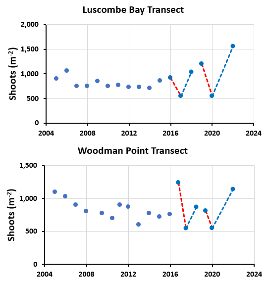
Figure 4: Seagrass shoots per square metre in Cockburn Sound 

From the published seagrass shoot density data in Cockburn Sound (WAMSI-Westport, 2024), it appears that the maximum density is approximately 1,600 shoots/m². Assuming this maximum corresponds to 100 % seagrass cover, it appears that the seagrass cover in Cockburn Sound ranges from 30 to 75 % of the seabed. The peak is similar to seagrass cover in Corio Bay.

From these examples, and an examination of long-term seagrass monitoring data from other sites, it is concluded that:

• Seagrass cover (or an equivalent metric) should be determined at least annually;
• Seagrass cover is the metric recommended as it records an estimate of seagrass biomass and therefore the volume of seagrass contributing to primary productivity and extracting carbon dioxide;
• An “impact” effect can be distinguished from the effects of other processes when reference sites are used;
• As there can be large variations from year to year, long-term monitoring is desirable.

It is apparent that a cost-effective monitoring procedure is required because of the extensive seagrass monitoring that is required to document whether or not an impact has occurred. 

Example of use of drone image method

Seagrass cover determined from underwater images has been used to assess  the effects on seagrass cover of effluent discharges from wastewater treatment plants, brine discharges, industrial discharges and dredging in Port Phillip Bay.  

Recently, an assessment was made of the potential impact of a cooling water discharge from a refinery in Corio Bay, which is on the western edge of Port Phillip Bay. The cooling water has been discharged into the shallow water for 60 years; therefore any effects on seagrass should be well-established. The warm water plume is generally in nearshore waters less than 2 m deep. Therefore, seagrass cover calculated from drone images were used to determine whether the cooling water discharge has had a significant effect on seagrass condition.

North Corio Bay was divided into two zones to assess whether there was a significant difference in seagrass cover between the area covered by the plumes (west zone) and a reference zone well away. Each zone was approximately 1 km long, in the shallow waters parallel to shore, as shown in Figure 5. The comparison was made for both subtidal seagrass (dense H. nigricaulis mixed with small patches of Althenia and occasional patches of Halophila) and intertidal seagrass (Nanozostera muelleri), with the results summarised below.

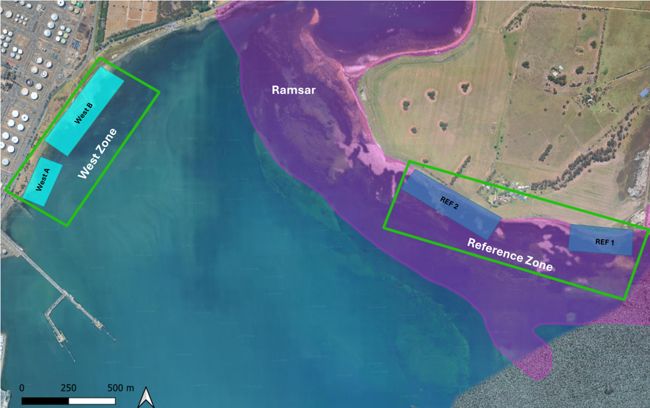
Figure 5: Location of survey areas in West Shore and Reference zones

Four transects were designated in each zone along selected depth contours (to 2 m depth) and 4 m² quadrats were defined at 15 m intervals along the transects. Seagrass cover was determined in each quadrat using the classifications listed in Table 1. To understand seasonal effects, three sets of zone images were taken at two-month intervals. 

An analysis of the three sets of images showed there were seasonal variations in the amount of seagrass cover in individual quadrats (due to swans feeding, disease, sediment movement or other factors) but that the average seagrass cover along each transect remained the same.

The cooling water discharge and plume occupied most of the west zone whereas the reference zone was well away (and in the Bellarine Peninsula Ramsar Site, DELWP 2018) with no cooling water plume. The most direct comparison was therefore to compare the distribution of seagrass cover on the transects in the two zones. The results are summarised in Figure 6.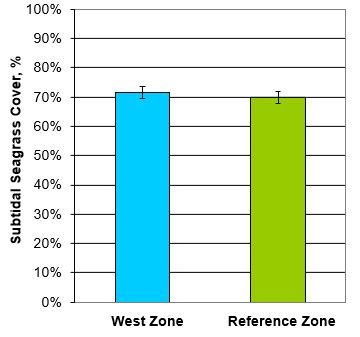  

Figure 6: Comparison of seagrass cover data

A total area of 1672 m² was assessed for seagrass cover in the west zone and the average seagrass cover was 72 % +/- 4 %. A total area of 1344 m² was assessed for seagrass cover in the reference zone and the average seagrass cover was 70 % +/- 6 %.  

The difference in subtidal seagrass cover between the West and Reference zones is 1.6 %.  The combined SD = 4.6 %. The two-sided t-value for the data is 0.7. The p-value is 0.56. The difference in subtidal seagrass cover is not significant at P < 0.05. In conclusion, the two-sided t-test shows there is no significant difference between the average seagrass cover in the two zones in north Corio Bay.

A second comparison using analysis of variance was used to test whether zone and time had a significant statistical effect. The test statistic (F) is 0.49, the square of the t-value of 0.7, and confirming that there is no significant difference between the average seagrass cover in the two zones of north Corio Bay, and no apparent effect on seagrass from the cooling water discharges.   
Another possible factor is a trend in seagrass cover along the transects – specifically with distance from the cooling water discharges. This was checked by fitting a line of best fit to seagrass cover values along a transect. The correlation coefficient between seagrass cover and distance was 0.005 – that is, a negligible correlation.

Averaging the results in the two zones from the drone images shows that  the average seagrass cover in north Corio Bay in 2023 was 71 % (ie, the patches of bare seabed between seagrass plants account for 29 % of the seabed). This is characteristic of seagrass meadows, where there rarely is 100 % cover over the whole zone. 

The same procedure was used to determine if there was an impact of the cooling water discharge on intertidal seagrass. As the cooling water plumes are buoyant (like freshwater effluent plumes), the intertidal seagrass near the discharge is regularly within the plume. Three surveys for the intertidal seagrass in each of the West and Reference zones was made using drone images and the seagrass cover classification procedure.

A total intertidal area of 1080 m² was assessed for seagrass cover in the west zone and the average seagrass cover was 31 % +/- 5 %. A total intertidal area of 1,128 m2 was assessed for seagrass cover in the reference zone, with an average seagrass cover of 30 % +/- 5 %.   Intertidal seagrass is more sparse and patchy than subtidal seagrass. A two-sided t-test showed a p-value is 0.68. The difference in seagrass cover is not significant at p < 0.05. In conclusion, there is no significant impact on the intertidal seagrass cover either.

It is concluded that the presence of the warm water discharge plumes does not have a significant impact on intertidal seagrass cover.

Discussion

Repeatability of classification

To check the repeatability of the seagrass cover classifications, the classification was repeated one month later for four transects in the October 2023 survey. For the subtidal transects, the mean seagrass cover from the second classification differed from the mean seagrass cover in the first classification by +/- 1.0 %. For the intertidal transects, where there was more spatial variability, the mean seagrass cover from the second classification differed from the mean seagrass cover in the first classification by +/- 1.8 %. 

As the shifts in the mean cover values are much smaller than the 95 % confidence intervals of the mean for the subtidal seagrass comparison (which is -12 % to 8.3 % cover) and the intertidal comparison (-9 % to 12 % cover), it is concluded that the results are not sensitive to the adopted classification procedure.

Causes of natural variability in seagrass cover

The location, depth and density of seagrass are subject to change over time due to variations in weather, floods, droughts, turbidity, nutrient inputs, diseases, grazing by swans and sea urchins, and other factors. Thus, seagrass cover has large natural variations from year to year. Additional factors influencing seagrass growth and development are wave-induced erosion, sediment movement and, for intertidal seagrass, accumulation of seagrass and algal wrack on the shore.

Seagrass roots (stolons and rhizomes) are the main food source for black swans (Swan Bay Environment Association, 2024). There are hundreds of black swans in Corio Bay, including those often eating seagrass in the cooling water plumes. It is estimated that the swans could consume up to 900 kg/d of seagrass, which would account for some of the local patchiness in the seagrass meadows (CEE, 2024). Consumption of seagrass by sea urchins and the effects of fungal diseases seen on H. Nigricaulis stems are other causes of local patchiness of seagrass. 

Conclusion

This study developed a method to measure percentage seagrass cover, taking into account the spatial variations in seagrass, seasonal variations and the change in seagrass species with depth.

Seagrass is naturally patchy and the location and size of seagrass patches vary over time. The monitoring of seagrass must take this patchiness into account and the seagrass cover calculated from drone images or underwater camera images meets this requirement.

The drone method allows large quadrats to be used and makes use of the high precision of position fixing in modern drones. The drone photographs can be obtained at significantly lower cost than underwater camera photographs.

Different water agencies and regulatory authorities have different preferences for monitoring seagrass and all the seagrass monitoring methods described above can achieve a satisfactory result. The drone method offers a cost-effective procedure for long term monitoring of seagrass conditions by the water industry.

Acknowledgements

Lywn Roberts conducted the drone photography and orthophoto rectification. Merric Northey assisted with seagrass and algal identifications. The fieldwork was partly funded by Viva Energy, who obtained clearances for drone surveys in Corio Bay.  

The Authors

Ian Wallis
Ian Wallis is a civil and environmental engineer with 35 years of experience in coastal and estuarine studies in all States and Territories of Australia. He was an EPA environmental auditor for 12 years and served on the Board of an EPA for 7 years. He was on the Expert Committee for Dredging. He has been on several environmental reviews for desalination projects. 

Nick Goodwin
Nick Goodwin is an environmental engineer with over seven years’ experience in environmental impact assessment and marine ecology. He has experience in seagrass mapping and analysis, water quality monitoring and industrial water discharge assessments across Victoria’s coastal environments.  

Scott Chidgey
Scott Chidgey is a marine scientist with more than 25 years of consulting experience in multidisciplinary marine studies throughout Australia, Timor Sea, Gulf of Papua and Pacific islands. Seagrasses are an important ecological and environmental value in many of these projects. He works closely with engineers and other scientists from a range of organisations.  

References

Ball, D, Sokolov-Berlson and P Young (2014). “Historical seagrass mapping in Port Phillip Bay, Australia”. J Coast Conserv (2014) 18:257-272.
Blake S and D Ball (2001) “Seagrass Mapping Port Phillip Bay”. Marine and Freshwater Resources Institute Report No. 39, Queenscliff, Australia
Ball. D, Parry. G, Heislers. S, Blake. S, Werner. G, Young. P, Coots. A (2010). “Victorian Multi-Region Seagrass Health Assessment”, Fisheries Victoria.
BMT (2023) “Port of Brisbane Seagrass Monitoring Program Report 2023 (also earlier years).
Cambridge, M and McComb, A (1984) “The loss of seagrasses in Cockburn Sound, Western Australia”, Aquatic Botany, Vol 20 pp 229-243.
CEE (2024) “Results of Three Seagrass Surveys in Corio Bay” Technical Memorandum on Seagrass Study.
Cockburn Sound Management Council (2021) “Annual Environmental Monitoring Report”
CSIRO (1996). “Port Phillip Bay Environmental Study Final Report”
DELWP (2018). “Port Phillip Bay (Western Shoreline) and Bellarine Peninsula Ramsar Site Management Plan”.
Duarte, C. M. (1991). “Seagrass depth limits”. Aquat. Bot. 0: 363-377.
Dennison WC, et al. (1993) “Assessing water quality with submerged aquatic vegetation”. Bioscience 43:86 –94
Eigenraam. M, McCormick. F, and Contreras. Z (2016). “Marine and Coastal Ecosystem Accounting: Port Phillip Bay”, Report to the Commissioner for Environmental Sustainability.
EPA SA (1998). Changes in Seagrass Coverage. EPA Report.
EPA VIC (1997) “Bulletin 588”
Hirst A, D Ball and S Blake (2012). “Baywide Seagrass Monitoring Program – Milestone Report No 15”, Fisheries Victoria Technical Report No 164, Feb 2012.
James Cook University (2024). “Seagrass meadows face uncertain future” March 2024.
Jenkins G, Keough M, Ball D, P Cook, A Ferguson, J Gay, A Hurst, R Lee, A Longmore, P Macreadie, S Nayer, C Sherman, T Smith, J Ross and P York (2015). “Seagrass Resilience in Port Phillip Bay”, Final Report, DELWP
Larkum, A, Orth, R and Duarte, C (2006). “Seagrasses: Biology, Ecology and Conservation”. 10.1007/978-1-4020-2983-7_5.
Marine Education Society of Australia (2025) website accessed May 2025.
Orth R.J., Carruthers T.J., Dennison W., Duarte C., Fourqurean J., James R., Hughes A., Kendrick G., Kenworthy W., Olyarnik S., Short F., Waycott M. and Williams S. (2006). “A global crisis for seagrass ecosystems”. Bioscience 56:987-996
Marine Science & Ecology (2006). “Review of Impacts of Dredging Turbidity Plumes on Seagrasses in Corio Bay in the Geelong Arm Channel Improvement Program”, Report to Victorian Channels Authority
Port of Brisbane website (2025). “Environmental Monitoring – Seagrass”, 12 survey reports from 2006 to 2023.
Swan Bay Environment Association (2024) Website accessed 20 Oct 2024.
Walker, DI and McComb, AJ (1992). “Seagrass degradation in Australian coastal waters”, Marine Pollution Bulletin, Vol 25, 191-195.
WAMSI-Westport (2024) “Two Decades of Seagrass Monitoring Data show drivers include ENSO, Climate Warning and Local Stressors”.