


Climatic influences on Warragamba water quality
DOWNLOAD THE PAPER
Abstract
Understanding the role that a changing climate plays on the drinking water quality of Sydney’s water storage system is necessary for long term strategic supply planning. This study used Bayesian Hierarchical Models and water quality data from 2000 to 2022 from within Warragamba Dam (~80% of Sydney’s drinking water storage), to quantify long term trends in water quality and the strength of climatic influences through rainfall and fire. The methods and outputs presented in this study are highly applicable to areas of future fire planning, climate scenario forecasting for water supply, catchment land management programs and water quality regulatory frameworks.
Introduction
Anthropogenic emissions induced changes to global climatic trends has impacted nearly all aspects of our environment. Of ubiquitous importance across all regions are the expected changes to the volume and quality of drinking water available for supply due to currently observed, and further expected alterations to historical weather patterns. The challenges posed by climate change to drinking water supply strategies is acutely highlighted within Australia, where rainfall patterns are highly varied both spatially and temporally, and which maintains the lowest mean yearly rainfall of any continent. Between 1999 to 2018 southeast Australian rainfall during the April to October period declined by around 11% when compared to the 1900 to 1998 period. In addition, the sum of the daily Forest Fire Danger Index for these regions has increased by around 10-20 points per year between 1997 to 2017 (State of the Climate 2022). As a background to this drying trend, extreme rainfall events have become more common with rainfall intensity directly linked to temperature’s effects on the water holding capacity of the atmosphere, i.e., for every degree of warming, total rainfall during storm events is expected to increase by approximately 7% (State of the Climate 2022).
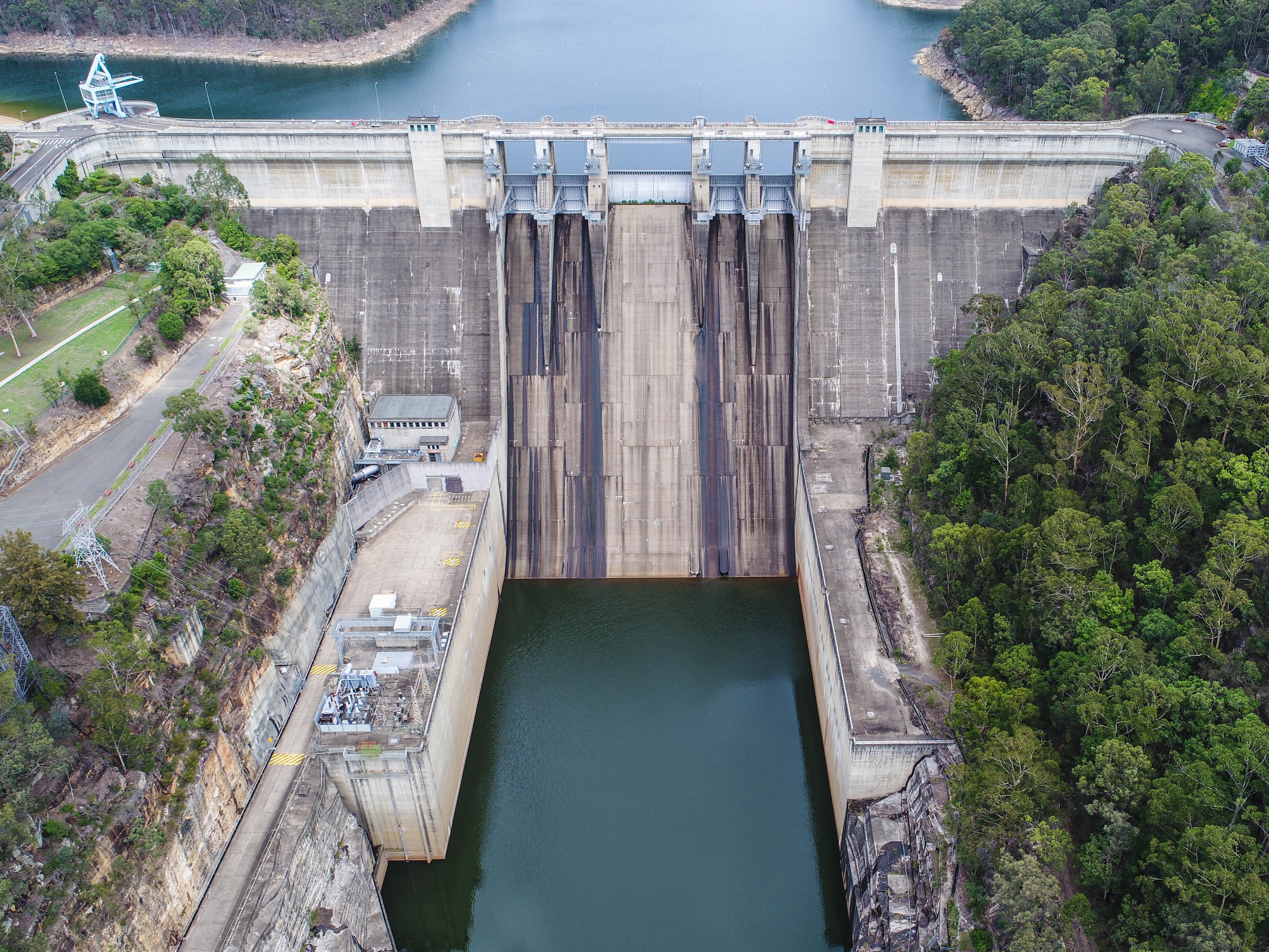
The southeastern areas of Australia are the most highly populated in the country, and have exhibited long term weather patterns conducive to compound weather events, where multiple weather factors interact to create particularly challenging conditions for drinking water storage and supply. In 2019, Sydney’s water supply was sitting at record low levels after a multi-year lower than average rainfall period. This led to exceedingly dry conditions in the catchment and an extensive build-up of dry plant materials, facilitating the 2019/2020 Black Summer fire season. This burnt ~9050 km2 of protected forested surrounding Lake Burragorang (Warragamba Dam), which is the source for about 80% of Sydney’s drinking water supply (Yang et al., 2020; Neris et al., 2021). Two weeks after the fires were contained an approximately one in forty-year rainfall event occurred, preceding one of the wettest two-year periods on record for Sydney’s Drinking Water Catchment (Boer et al., 2020; Yang et al., 2020; Neris et al., 2021).
The burning of vegetation and subsequent deposition of ash and soil materials into fluvial systems poses risks to drinking water quality, such as increased loads of nitrogen, phosphorous, trace metals, and organics (Lane et al., 2008; Wilkinson et al., 2009; Honer et al., 2019; Blake et al., 2020). The magnitude of these risks is a product of a range of interactions, including, the level of fire intensity (Chafer et al., 2004), total burned area (Chafer et al., 2004, Yang et al., 2020), the frequency and intensity of rainfall events (Neris et al., 2021), seasonal thermal stratification of the lake (Pearl & Scott 2010), sediment intrusion transport dynamics (Pearl & Scott 2010), and the chemical fate of fire related constituents (Wilkinson et al., 2011).
Understanding the role that a changing climate has played on the source water quality of Sydney’s water supply systems is necessary for long term strategic supply planning, and the maximisation of benefits from in-catchment land management activities. This paper analyses 22 years of water quality data from 2000 to 2022. The sampling point selected was 500 metres from the Warragamba Dam water offtake point, and data was analysed to establish long term trends in water quality and their links to the climatic influences of fire and rainfall. We use Bayesian hierarchical models to estimate the linear changes in water quality parameters over time, separating out background effects of rainfall and fire from general trends, establishing a quantitative summary of historical climatic influence on Sydney’s drinking water supply.
Methods
General summary
All routine and special samples were taken from the WaterNSW Water Quality Data Base through PowerBI, for the period of 1-January-2020 to 1-January-2022. Water quality parameters analysed included; Algal biovolume (mm3 L-1), cyanobacterial biovolume (mm3 L-1), algae (areal standard unit), cyanobacteria (areal standard unit), aluminium filtered (mg L-1), aluminium total (mg L-1), conductivity (mS cm-1), iron filtered (mg L-1), iron total (mg L-1), manganese filtered (mg L-1), manganese total (mg L-1), nitrogen total (mg L-1), organic carbon dissolved (mg L-1), organic carbon total (mg L-1), pH, true colour (TCU at 400nm) and turbidity (NTU). Where multiple names for the same parameter were found in the database (i.e., pH, pH Lab-Field, Lab/Field), all data columns were combined into one variable for analyses. Individual data frames were created for each analyte, all missing/blank values and all zero values were converted to NA, with all cells containing NAs subsequently being removed from all data frames.
Common in water quality concentration data is the presence of left censored values that are lower than the reportable limit (LRL) of sampling equipment, with this lower limit often changing through time as sampling technology changes. To impute LRL values across the data period, all samples displaying a less than symbol were run through an automatic number generating loop that randomly sampled from a uniform probability distribution between the known data limit of zero, and the LRL limit of the respective datapoint (Pleil, 2016).
Each analyte was cleaned of outliers through a conservative Cook’s Distance cut-off of >0.85 (McDonald 2002) so as to include as much natural variation as possible in analyses, while pruning the data of data entry errors orders of magnitude distant from the data modelled mean (“cooksd()” function, within the “car” package) (Cook 1986; McDonald 2002).
Statistical analyses were performed in R-statistics, packages are listed after their function as described below.
Reservoir specific data treatment
Data from Warragamba Reservoir, 500m from dam wall (site code DWA2), was structured available as weekly, or fortnightly, single point source concentration samples within each of the routine sampling depth ranges; 0-6m, 6-9m, 9-12m, 12-18m, 18-24m, 24-36m, 36-48m, 48-60m, and 60-84m. Where a composite sample existed in the data it was used instead. The point source samples were assumed as the concentration for the entire depth increment.
To obtain a single representative parameter concentration value for each sampling date for use in whole-reservoir trend analyses, a mass balance equation was used to simulate a homogenously mixed water column. Note, algal analytes were not mixed, instead the top 0-12m were used. Mass-balance mixing methods produce a more robust estimate of a pseudo reservoir average, as it accounts for volume changes along with concentration changes (i.e., high manganese in deeper, lower volume, portions of the lake profile would disproportionately affect an average term exclusive of volume).
To estimate a mixed concentration, analyte masses were calculated for each depth increment and divided by the respective total reservoir volume to simulate water column mixing, as described in Equation 1. This method is subject to two main assumptions, (1) Depth-based concentrations at the dam wall are assumed as representative of the depth-based concentrations of the whole reservoir; and (2) The lake is fully homogenised/mixed. These assumptions are of low consequence to this study, as here we are not attempting to predict a mixed concentration, but instead obtain a pseudo average value normalised to volume for trending across years.
Equatation 1:

Where analyte α represents the estimated concentration of an analyte after full mixing, Total V represents the total volume stored within the reservoir at the time of sampling, di represents the number of sampling depth intervals in the reservoir (e.g. nine for Warragamba), Vi represents the volume of each depth increment between sampling points as obtained from bathymetry data, while αD1i and αD2i represents the concentration of analyte α within the upper and lower samples of each depth increment respectively.
Burn data treatment
Both Hazard Reduction Burns (HRBs) and Wildfires contribute to water quality alteration through a range of processes including, thermal decomposition and release of chemicals stored in vegetation, increases in erosion due to the lowering of vegetive ground cover, and the deposition and subsequent resuspension of fire materials in waterways.
Historical data for all HRBs and Wildfires across the forested Warragamba Special Areas (~2600 km2) were obtained from the combined historical fires layer for NSW, extracted from NSW Rural Fire Service (Incident Coordination Online) ICON Database. Access to ICON burn data was facilitated by WaterNSW’ internal Spatial Modelling Team. Area burned in metres squared were summed for each year in the time series, irrelevant of burn type. Where no fire was recorded for the full year, a zero was used to represent the cumulative burnt area.
Previous studies in the Warragamba Catchment have demonstrated that fire-related materials remaining in the catchment can pose risks to water quality for 3-5 years post fire-event through ongoing fluvial transport and distribution (Wilkinson et al. 2011). To conservatively account for inter-year fire contributions to water quality trends, a ‘Fire Proxy’ value was produced that assumed a continued 25% influence of burnt area on water quality from one year prior, and a 10% effect from two years prior, in accordance with the below Equation 2.
Equatation 2:
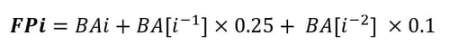
Where FP represents the Fire Proxy value expressed in m2, BA represents a cumulative Burnt Area value expressed in m2, and i represents the year of calculation.
Rainfall data treatment
To incorporate background weather patterns into modelling of water quality trends, the average daily rainfall (mm) across Warragamba catchment was used (col361 Daily Returns, Data Download). Rainfall data is an average of 210 collection sites across Lake Burragorang Catchment (Figure 1). The daily rainfall values were summed to a total yearly rainfall value (mm).
 Figure 1: Distribution of rainfall gauges across the Lake Burragorang Catchment. Note, rain gauges periodically undergo maintenance and as such some may be included in historical data for short periods.
A prior understanding of water quality changes in large reservoirs is that impacts from large rainfalls can continue to affect parameter concentrations for a period of months post-event, e.g., a large rainfall event in November[Yeari] is likely to contribute to increased organic compounds present in February[Yeari + 1]. To account for ongoing rainfall contributions to water quality, a proxy rainfall value was estimated that incorporated a continued 25% influence of rainfall from one to six months prior, and a 10% influence of rainfall from six to twelve months prior, in accordance with the below Equation 23. The magnitude of residual influence from previous rain was assumed in this study, further work could improve the accuracy of these values.
Equatation 3:
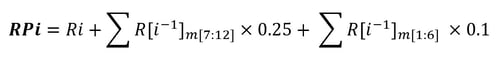
Where RP represents the Rainfall Proxy value expressed in millimetres, R represents a cumulative Rainfall value expressed in millimetres, i represents the year of calculation, and m represents the month as a value one to twelve.
Statistical analyses
Model structure
To analyse long-term trends in water quality, a Bayesian hierarchical generalised linear model was implemented using the ‘brm()’ function, within the “brms” package for R Statistical Software (Bürkner, 2017). Unlike frequentist statistical approaches that assume parameters of a model to be fixed (i.e., a single slope parameter for relationships between the dependant and independent variables), in Bayesian statistics parameters are incorporated as a distribution of probable values and are therefore more intuitively interpreted within risk assessment and decision-making frameworks. The brm() function links to the Stan program to implement Hamiltonian Monte Carlo No U-Turn Sampling of the probable posterior model distributions (Duane et al. 1987; Neal 2011; Hoffman & Gelman 2014).
Models were run for each analyte, with the dependent Analyte variable assessed against the independent Year of sample variable, Rainfall Proxy variable, and Fire Proxy Variable (see section 3.3 and 3.4 for calculation of these proxies). A smoothing term (also known as a spectral analysis) was placed on the month of sample collection to account for seasonal oscillations in analyte concentrations (12 knots for each month of the year, cyclic cubic regression splines), (Pedersen et al. 2019). Smoothed seasonal terms help prevent bias in the estimated yearly mean when samples are unevenly sampled throughout all seasons.
Model selection was performed using approximate leave-one-out cross validation with Pareto-Smoothed importance sampling with an estimated difference in model predictive accuracy in the form of an expected log pointwise predictive density (ELPD)(‘loo_compare()’ function, within the ‘brms()’ package) (Vehtari et al. 2017). Model selection started with the most simple model of the expected relationship, being that of a linear regression, and then combining more complexities such as seasonal smoothing, autoregressive terms applied to each sample date, variance heterogeneity, and likelihood distribution alterations. Aluminium Filtered (mg/L) was used as the representative analyte for model selection as it is highly abundant across all sites and evenly sampled across the time series of 2000-2022. The model selection summary for Warragamba Reservoir can be found in Supplementary Table 1.
The best model fit contained a Weibull likelihood distribution with a logarithm link to the linear model, the Weibull (log-link) is similar to a gamma (log-link) distribution and is highly flexible along the positive value scale. The Weibull distribution is often used in water quality studies as it assumes positive only data, and allows for increasing data variance with higher values (e.g., storm and inflow event concentrations compared to routine sampling concentrations) (Antonopoulos et al., 2001; Lee et al., 2008; Krueger 2017). In addition, a log-link model reduced the need for data transformation to achieve normal distribution of residuals, hence in this study no transformations were performed on raw data. Due to the log-link of the Weibull distribution, the slope parameter of the model outputs are expressed as a percentage change in the dependant variable with every one unit increase in the independent variable.
Model fits were validated by ensuring that trace plots of the four independent Markov-Chain Monte-Carlo (MCMC) chains mixed well (‘trace’), histograms of posterior parameter draws were normally distributed (‘hist’), boxplots of observed values were qualitatively homogenous with simulated datasets (‘boxplot’), leave-one-out probability integral transformation plots showed no distinct variation from the observed data (‘loo_pit’), and that the empirical cumulative distribution function closely matched that of the observed data (ecdf_overlay) (Gelman et al., 2013; Gabry et al., 2019)(Supplementary Figure 1a-e). No models were accepted that stated an error of R-hats greater than 1 (Bürkner 2017 & 2018).
Results
To establish the effects of rainfall and fire on long term trends, the slope of simple linear models (concentration vs time) was compared to more complex models with these climatic effects included (concentration vs time, rainfall and fire). The resulting change in slope expressed as a percentage indicates how much of the average over time change in water quality may be accounted for through changes in rainfall and burnt land mass. Rainfall and fire accounted for an average 78.5% of the across time variations in water quality concentrations when incorporated into time series models. For example, Turbidity (NTU) change over time was estimated at 2.5% yr-1 (1.51% – 3.49%, 95% CI)(Figure 2a) using a simple linear model that represents average change over time, however the disaggregation of this time trend from the climatic effects of rainfall and fire resulted in an updated over time estimate of negative -3.03% yr-1 (-4.13 – -1.93%, 95% CI) (Figure 2b & Figure 3).
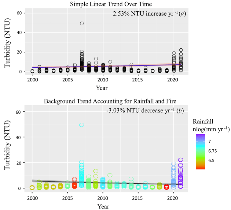
Figure 2: Turbidity (NTU) trends over time exclusive and inclusive of rainfall and fire, (a) and (b) respectively. Circular data points are representative of the estimated mixed turbidity concentration of Lake Burragorang (Equation 1), each circle is the amalgamation of a full depth profile for a single day within that year. Sample abundance over years is subject to alterations in historical sampling routines and special event sampling, however Bayesian analyses techniques are highly robust to these differences through estimation of probable distributions. These results show that while turbidity concentrations have trended upwards over time (a) these increases are due to large rainfall events, with improving background turbidity inputs relative to rainfall volumes (b).

Figure 3: Turbidity’s relationship to rainfall and fire. The interaction between rainfall and fire positively influences estimated turbidity, showing how large events in 2020 and 2021 are likely to have contributed towards overestimates of time’s effect within simple linear trends Figure 2(a). This interaction value infers that rainfall events in burnt catchments exert greater influence on turbidity concentrations, seen here where a 1300mm rainfall year’s estimated turbidity is ~10 NTU, while the same rainfall volume in a 500 km2 burnt area year results in an estimated doubling of the resulting turbidity.
Across all analytes tested, simple linear models showed probable mean concentration increases in 79% of analytes (determined as >95% probability of a positive slope), however, only 47% of analytes retained estimates of probable increasing concentration changes once rainfall and fire were accounted for. The mean change (slope) over time across all analytes, not attributed to rainfall volume or fire burnt area, was estimated at 1.93% ± 0.29% unit-1 yr-1.
The median estimated influence of rainfall (total yearly millimetres) on water quality concentrations was an increase of 0.29% mm-1 yr-1, ranging from -0.02% – 1.17% (95% CI) (Figure 4a) (i.e., an increase of 1mm rainfall within a given year resulted in an estimated analyte concentration increase of 0.29%). The interaction between rainfall and fire was substantively positive in 73% of analytes (>95% probability) (Figure 4b). Using the statistical parameters produced through these analyses we can estimate water quality changes using simulated environmental conditions, i.e., assuming rainfall in the year 2023 matches that of the 2000 – 2022 mean, a 2km2 burn (common yearly hazard reduction burn size) would increase turbidity (NTU) by 1.12% (0.73 - 1.48% CI) compared to no burns under the same conditions.

Figure 4: Frequency distribution of probable relationships between water quality parameters, Rainfall only Fig 3(a), and Rainfall-Fire interactions Fig 3(b) using a Bayesian Hierarchical Model. The distributions can be interpreted as a range of probable slope values given the data, with more probable slopes found at the median point of the distribution.
Rainfall had a positive effect on the concentrations of dissolved organic carbon (DOC) (0.06% mm
yr-1, 0.02% to 0.08% CI), total organic carbon (TOC) (0.05% mm yr-1, 0.02% to 0.08% CI), and true colour at 400nm (TC) (0.21% mm yr-1, 0.17% to 0.25% CI). However, the interaction terms between rainfall and fire attributed to these analytes were found to be negative at -0.002% mm-1*km2 (99.45% probability), -0.001% mm-1*km2 (99.4% probability), and -0.001% mm-1*km2 (80.92% probability), respectively, indicating fire reduced the loads of these analytes delivered through rainfall.
Conductivity (mS cm-1) was found to be increasing at a median of 1.05% yr-1 at the dam wall of Lake Burragorang. A linear increase in conductivity was found between 2010-2017 parallel to major rainfall events indicating potential anthropogenic inputs (Figure 5).

Figure 5: Conductivity trends in Lake Burragorang. Periods of freshwater inputs decrease conductivity by diluting the electrically conductive saline properties of the lake, however during the 2010-2017 period conductivity steadily increased (a) in parallel to major rainfall events (b), indicating potential anthropogenic inputs. Circular data points are representative of the estimated mixed conductivity concentration of Lake Burragorang (Equation 1), each circle is the amalgamation of a full depth profile for a single day within that year.
There were no statistically probable changes detected in algal and cyanobacterial biovolumes (mm3 L-1). To note is that algal data at the dam wall of Lake Burragorang (DWA2) was irregular, and year-long gaps exist which add to the lack of probable certainty in trends.
A complete list of all analyte parameters and model visualisations can be found in the attached Supplementary Material.
Discussion
Long term drinking water supply planning is a field highly reliant on the identification of changing catchment conditions and their subsequent influence on water quality and quantity. Ecological and physical properties of a catchment, such as extreme rainfall and fire events play a critical role in shaping water quality trends in reservoirs, however, quantification of these dynamics are currently lacking. Using a temperate reservoir case-study within south-eastern Australia, and Sydney’s largest water storage system, we quantitatively demonstrate that rainfall and fire events substantially influence estimated water quality change over time. As further described below, this study showed that an estimated 78.5% of water quality concentration changes analysed between 2000-2022 can be attributed to large rainfall and fire events towards the end of this period, i.e., concentrations within inflows have on average reduced over time, large inflow volumes have counteracted these concentration reductions. In addition, we show that the interactive effects of rainfall and fire vary in importance across key water quality analytes and discuss residual conductivity trends in the context of anthropogenic inputs.
The 2019/2020 black summer fires and subsequent flooding events across south-eastern Australia correlated with large changes in Lake Burragorang water quality, which supplies ~80% of Sydney’s drinking water (Yang et al., 2020; Neris et al., 2021). The standard methods for investigating long term water quality change in Sydney’s catchment is through a biannual review using a combination of mean or median change, analyte-specific threshold breaching event abundance, and Mann-Kendall-Sneyers (MKS) time series analyses (Mann 1945; Sneyers 1991). However, these methods do not account for the increasingly common effects of large rainfall and fire events, potentially leading to an overestimate of background change attributed to non-climatic catchment conditions. With millions in funding allocated annually across Sydney’s drinking water supply catchments towards optimal land management practices for water supply, correctly quantifying and categorising influencing factors into the effects of a changing climate (i.e., rainfall and fire combined) and the effects of a changing catchment (e.g., vegetation change, agricultural inputs etc) ensures mitigation program efficacy, and more accurate long term supply planning. Here we find that in comparison to simple linear models, and across all analytes tested, mean rate of water quality change over time reduced by 78.5% when rainfall and fire were incorporated into the model. This finding more accurately represents changes in catchment conditions, outside of climatic events, and allows for further informed investigation of residual change in the context of land management programs. In addition, this result highlights the necessity for long-term water supply planning to take into account multiple climate scenarios, and the quantifiable impacts of major climatic events, on water quality and treatment capacity for effective management.
The statistical method used in this study allows for enhanced estimation of future water quality conditions based on current conditions, assumed yearly rainfall, and assumed yearly fire. For instance, a simple linear model using turbidity (NTU) concentrations over time estimated a yearly increasing trend of 2.56% over the study period, while the hierarchical model applied here which disaggregates climatic effects to estimate slope parameters for time, rainfall and fire, resulted in a reducing yearly trend of -3.05%. This disaggregated hierarchical model established that historical fluxes in turbidity were attributed to concurrent inflow and fire events. Therefore, using the statistical parameters produced through these analyses we can estimate water quality changes using simulated environmental conditions, i.e., assuming rainfall in the year 2023 matches that of the 2000 – 2022 mean, a 2km2 burn (common yearly hazard reduction burn size across the Lake Burragorang Catchment) would increase turbidity (NTU) by 1.12% (0.73 - 1.48% CI) when compared to no burns under the same conditions. This statistical forecasting provides multiple lines of evidence for other process/conceptual models commonly applied to catchment and in-lake processes across Australia, and aids in both the decisions of land programs and preparation for treatment options.
Just under half (47%) of the analytes tested in this study continued to show background concentration changes outside of the direct climatic effects of rainfall and fire. Here we discuss two main potential causes of these increases, Regime Shifts, and Changes of Inflow Concentrations. However, note that within highly stochastic catchment scale ecosystems, time-based trends are often the product of multiple compounding biological, geophysical, and chemical interactions.
Regime shifts in the environment describe when a substantial ecosystem shift occurs due to new or ongoing variations in environmental conditions, this can occur when either the strength of the conditional change is large enough, or the time between condition change events becomes small enough, that the system no longer rebounds and can be characterised at a significantly different baseline (Anderson et al., 2009; Hilt et al., 2011; Hilt et al., 2017). For example, photodegradation of chemicals and benthic settling of particulates are two major components that contribute towards ecological elasticity in freshwater lakes, however, these processes have a natural maximum rate depending on the system and thus can be outbalanced by multiple large inputs of lower quality. Understanding the potential regime shifts that may have occurred within the timeseries of this study through event categorisation could help to disentangle the reasons behind background concentration increases, and possible management actions that facilitate increased ecological elasticity. And,
Changing inflow concentrations. While the analysis method used in this study accounts for changing rainfall volumes, it does not account for changing inflow concentrations. The planned next stage of this study is a flow normalised trend analyses for inflow sites across Lake Burragorang, that aims to determine if the mass, or load, of key analytes have changed over time. A detected across time change in input load under similar rainfall conditions, could be indicatory of changing catchment conditions (e.g., land-use in unprotected areas or natural vegetation change), helping to inform targeted management response.
Across 73% of analytes studied, rainfall and fire were shown to share a probable increasing multiplicative relationship with each other (>95% probability). This interaction term represents the multiplicative relationship between rainfall and fire, where burns accompanied by rainfall may have a far greater effect on water quality due to run-off of thermally degraded ash materials during rainfall events, when compared to equally wet years with no fire. Interestingly, while rainfall alone had an increasing effect on the concentrations of dissolved organic carbon, total organic carbon, and true colour (at 400nm), the interaction term between rainfall and fire attributed to these analytes was negative. These findings suggests that counter to previous expectations, fire may reduce the available organic material in run-off through thermal volatilisation (release to the atmosphere as a gas) of previously chemically leachable litter materials (Gray & Dighton 2006; Neris et al., 2021). Large inflow years across the analyses period qualitatively contributed the same or more organics when no fire was present, which in combination with a lack of rainfall fire interaction, indicates that within Lake Burragorang reservoir, fire did not increase organic matter and colour concentrations.
Conductivity (mS cm-1) was found to be increasing at 1.05% yr-1 at the dam wall of Lake Burragorang. Freshwater lake conductivity naturally decrease during inflows, and increase during dry periods where evaporation leads to greater salinity and therefore electrical conduction (Williams 2001; Alcocer & Filonov 2007; Marotta et al., 2010). Freshwater lakes naturally become more saline over large periods of time, through both rainfall from saltwater origins, and run-off that has filtered through mineral rich soils and rocks (Webster et al., 2000). However, outside of natural salt biogeochemical cycling, recent literature has shown that anthropogenic activities such as human-accelerated weathering, sewage, fertiliser, and mine drainage have contributed to increased salinity in drinking water reservoirs, termed global Freshwater Salinisation Syndrome (FSS) (Cañedo-Argüelles et al., 2013; Herbert et al., 2015; Kaushal et al., 2018; Reid et al., 2019). An increasing concentration trend in conductivity during the higher than average rainfall period of 2010-2015 (Figure 4) may indicate previous anthropogenic saline inputs in Lake Burragorang. Further assessment is required to determine if the former is the root cause of this trend or if a combination of natural lake processes and anthropogenic pressures are at play. Planned trend analysis on major inflow streams will help identify the contributing factors to these trends in Lake Burragorang.
Conclusion
In conclusion, this study provides quantitative data on extreme climatic event’s adverse effects on raw water quality of south-eastern Australia, finding that commonly used water quality trend analysis methods are inaccurate in the inference of changing drinking water catchment conditions. We find that over the 2000-2022 period the combined effects of rainfall and fire accounted for an estimated 78.5% of water quality concentration changes in Sydney’s largest drinking water supply reservoir. In addition, we demonstrate the use of Bayesian hierarchical modelling tools for the identification of background catchment associated water quality trends, highlighting that commonly used simple linear trend analysis techniques vastly under-estimate the positive effects of land management activities across catchments by ignoring changing climatic conditions. We also find that counter to original hypotheses, the burning of vegetation during fire years did not have a substantial effect on concentrations of dissolved organic carbon, total organic carbon, or true colour (400nm), (although fire followed by rainfall did impact the other parameters examined) with rainfall instead being the singular driver of these parameters. The analysis technique and outputs of this study are highly relevant to the design and assessment of both fire mitigation planning, and climate scenario forecasting for water supply, while the outputs are directly applicable to southeast Australian drinking water catchment land management programs.
The Authors
Quinn Ollivier
Experienced in the leadership of environmental management projects. Key areas of expertise include carbon accounting and water supply risk, the implementation of catchment-scale research projects with a focus on aquatic systems, statistical solutions, and extensive engagement of stakeholders within the private industry, academic and government sectors.
Lorena Oliveira
With almost 20 years experience in the water sector, I have had the opportunity to contribute to and lead initiatives spanning across the water cycle, from water recycling to bulk water supply, and from metropolitan areas to remote regional services. I bring leadership experience in people management, governance, program management (large capital and R&D portfolios), strategic planning and operational risk management. Qualifications: Bachelor of Sanitary and Environmental Enginering (UFSC-BR) and a Master of Engineering Science (UNSW-AU).
Dr Lisa Hamilton
Dr Lisa Hamilton is a Research and Innovation Manager with a breadth of applied research experience across the water industry including water quality in catchments, estuaries, wastewater treatment and potable distribution systems. Lisa has a PhD specialising in ecotoxicology and wastewater treatment and has industry experience in the evaluation of anthropogenic impacts on aquatic ecosystems and guiding management interventions for the protection of water quality and ecosystem function.
References
Andersen, T., Carstensen, J., Hernandez-Garcia, E., & Duarte, C. M. (2009). Ecological thresholds and regime shifts: approaches to identification. Trends in Ecology & Evolution, 24(1), 49-57.
Alcocer, J., & Filonov, A. E. (2007). A note on the effects of an individual large rainfall event on saline Lake Alchichica, Mexico. Environmental Geology, 53, 777-783.
Antonopoulos, V. Z., Papamichail, D. M., & Mitsiou, K. A. (2001). Statistical and trend analysis of water quality and quantity data for the Strymon River in Greece. Hydrology and Earth System Sciences, 5(4), 679-692.
Blake, D., Nyman, P., Nice, H., D’Souza, F. M., Kavazos, C. R., & Horwitz, P. (2020). Assessment of post-wildfire erosion risk and effects on water quality in south-western Australia. International Journal of Wildland Fire, 29(3), 240-257.
Boer, M. M., Resco de Dios, V., & Bradstock, R. A. (2020). Unprecedented burn area of Australian mega forest fires. Nature Climate Change, 10(3), 171-172.
Bürkner P. C. (2017). brms: An R Package for Bayesian Multilevel Models using Stan. Journal of Statistical Software. 80(1), 1-28. doi.org/10.18637/jss.v080.i01
Bürkner P. C. (2018). Advanced Bayesian Multilevel Modeling with the R Package brms. The R Journal. 10(1), 395-411. doi.org/10.32614/RJ-2018-017
Cañedo-Argüelles, M., Kefford, B. J., Piscart, C., Prat, N., Schäfer, R. B., & Schulz, C. J. (2013). Salinisation of rivers: an urgent ecological issue. Environmental pollution, 173, 157-167.
Chafer, C. J., Noonan, M., & Macnaught, E. (2004). The post-fire measurement of fire severity and intensity in the Christmas 2001 Sydney wildfires. International Journal of Wildland Fire, 13(2), 227-240.
Cook, R. D. (1986). Assessment of local influence. Journal of the Royal Statistical Society: Series B (Methodological), 48(2), 133-155.
Duane, S., Kennedy, A. D., Pendleton, B. J., & Roweth, D. (1987). Hybrid monte carlo. Physics letters B, 195(2), 216-222.
Gabry, J. , Simpson, D. , Vehtari, A. , Betancourt, M. and Gelman, A. (2019), Visualization in Bayesian workflow. J. R. Stat. Soc. A, 182: 389-402. doi:10.1111/rssa.12378
Gabry, J. , Simpson, D. , Vehtari, A. , Betancourt, M. and Gelman, A. (2019), Visualization in Bayesian workflow. J. R. Stat. Soc. A, 182: 389-402. doi:10.1111/rssa.12378
Gelman, A., Carlin, J. B., Stern, H. S., Dunson, D. B., Vehtari, A., and Rubin, D. B. (2013). Bayesian Data Analysis. Chapman & Hall/CRC Press, London, third edition. (Ch. 6)
Gray, D. M., & Dighton, J. (2006). Mineralization of forest litter nutrients by heat and combustion. Soil Biology and Biochemistry, 38(6), 1469-1477.
Herbert, E. R., Boon, P., Burgin, A. J., Neubauer, S. C., Franklin, R. B., Ardón, M., ... & Gell, P. (2015). A global perspective on wetland salinization: ecological consequences of a growing threat to freshwater wetlands. Ecosphere, 6(10), 1-43.
Hilt, S., Köhler, J., Kozerski, H. P., van Nes, E. H., & Scheffer, M. (2011). Abrupt regime shifts in space and time along rivers and connected lake systems. Oikos, 120(5), 766-775.
Hilt, S., Brothers, S., Jeppesen, E., Veraart, A. J., & Kosten, S. (2017). Translating regime shifts in shallow lakes into changes in ecosystem functions and services. BioScience, 67(10), 928-936.
Hoffman, M. D., & Gelman, A. (2014). The No-U-Turn sampler: adaptively setting path lengths in Hamiltonian Monte Carlo. J. Mach. Learn. Res., 15(1), 1593-1623.
Hohner, A. K., Rhoades, C. C., Wilkerson, P., & Rosario-Ortiz, F. L. (2019). Wildfires alter forest watersheds and threaten drinking water quality. Accounts of Chemical Research, 52(5), 1234-1244.
Kaushal, S. S., Likens, G. E., Pace, M. L., Utz, R. M., Haq, S., Gorman, J., & Grese, M. (2018). Freshwater salinization syndrome on a continental scale. Proceedings of the National Academy of Sciences, 115(4), E574-E583.
Krueger, T. (2017). Bayesian inference of uncertainty in freshwater quality caused by low-resolution monitoring. Water Research, 115, 138-148.
Lane, P. N., Sheridan, G. J., Noske, P. J., & Sherwin, C. B. (2008). Phosphorus and nitrogen exports from SE Australian forests following wildfire. Journal of Hydrology, 361(1-2), 186-198.
Lee, K. S., & Kim, S. U. (2008). Identification of uncertainty in low flow frequency analysis using Bayesian MCMC method. Hydrological Processes: An International Journal, 22(12), 1949-1964.
Mann, H. B. (1945). Nonparametric tests against trend. Econometrica: Journal of the econometric society, 245-259.
Marotta, H., Duarte, C. M., Pinho, L., & Enrich-Prast, A. (2010). Rainfall leads to increased pCO 2 in Brazilian coastal lakes. Biogeosciences, 7(5), 1607-1614.
McDonald, B. (2002). A teaching note on Cook’s distance-a guideline, Research Letters in the Information and Mathematical Sciences, 3, 122-128.
Neal RM (2011). “MCMC Using Hamiltonian Dynamics.” In S Brooks, A Gelman, GL Jones, XL Meng (eds.), Handbook of Markov Chain Monte Carlo. Chapman & Hall/CRC. doi: 10.1201/b10905-6.
Neris, J., Santin, C., Lew, R., Robichaud, P. R., Elliot, W. J., Lewis, S. A., ... & Doerr, S. H. (2021). Designing tools to predict and mitigate impacts on water quality following the Australian 2019/2020 wildfires: Insights from Sydney’s largest water supply catchment. Integrated Environmental Assessment and Management, 17(6), 1151-1161.
Paerl, H. W., & Scott, J. T. (2010). Throwing fuel on the fire: synergistic effects of excessive nitrogen inputs and global warming on harmful algal blooms.
Pedersen, E. J., Miller, D. L., Simpson, G. L., & Ross, N. (2019). Hierarchical generalized additive models in ecology: an introduction with mgcv. PeerJ, 7, e6876. https://doi.org/10.7717/peerj.6876
Pleil, J. D. (2016). Imputing defensible values for left-censored ‘below level of quantitation’(LoQ) biomarker measurements. Journal of breath research, 10(4), 045001.
Reid, A. J., Carlson, A. K., Creed, I. F., Eliason, E. J., Gell, P. A., Johnson, P. T., ... & Cooke, S. J. (2019). Emerging threats and persistent conservation challenges for freshwater biodiversity. Biological Reviews, 94(3), 849-873.
Sneyers, R. (1991). On the statistical analysis of series of observations (No. 143).
State of the Climate 2022 – Australia continues to warm; heavy rainfall becomes more intense (2022) CSIRO. Commonwealth Scientific and Industrial Research Organisation. Available at: https://www.csiro.au/en/news/News-releases/2022/State-of-the-Climate-Report-2022 (Accessed: February 2, 2023).
Vehtari, A., Gelman, A., and Gabry, J. (2017). Practical Bayesian model evaluation using leave-one-out cross-validation and WAIC. Statistics and Computing. 27(5), 1413--1432. doi:10.1007/s11222-016-9696-4 (journal version, preprint arXiv:1507.04544).
Webster, K. E., Soranno, P. A., Baines, S. B., Kratz, T. K., Bowser, C. J., Dillon, P. J., ... & Hecky, R. E. (2000). Structuring features of lake districts: landscape controls on lake chemical responses to drought. Freshwater Biology, 43(3), 499-515.
Wilkinson, S. N., Wallbrink, P. J., Hancock, G. J., Blake, W. H., Shakesby, R. A., & Doerr, S. H. (2009). Fallout radionuclide tracers identify a switch in sediment sources and transport-limited sediment yield following wildfire in a eucalypt forest. Geomorphology, 110(3-4), 140-151.
Wilkinson, S., Wallbrink, P., Blake, W., Shakesby, R., & Doerr, S. (2011). Using Tracers to Assess the Impacts of Sediment and Nutrient Delivery in the Lake Burragorang Catchment Following Severe Wildfire. Soil Conservation Measures on Erosion Control and Soil Quality, 49.
Williams, W. D. (2001). Anthropogenic salinisation of inland waters. In Saline Lakes: Publications from the 7th International Conference on Salt Lakes, held in Death Valley National Park, California, USA, September 1999 (pp. 329-337). Springer Netherlands.
Yang, X., Zhang, M., Oliveira, L., Ollivier, Q. R., Faulkner, S., & Roff, A. (2020). Rapid assessment of hillslope erosion risk after the 2019–2020 wildfires and storm events in Sydney drinking water catchment. Remote Sensing, 12(22), 3805.
Supplement Material
Supplementary Table 1: Model selection outputs for Warragamba Reservoir and Aluminium Filtered (mg/L) using leave-one-out (LOO) cross validation. ‘bf()’ represents the bayesian formula for hierarchical model analyses as set out in ‘brms()’ package, ‘s()’ is a smoothing function applied to the seasonal variable.

Supplementary Table 2: Posterior predictive checks, a) Trace Plot, b) Histogram of parameter distributions, c) Boxplot of observed and simulated data, d) LOO-PIT plot of model fit, and e) ecdf-overlay of observed and predicted values.


Share